k-Means clustering
set.seed(90210)
kmodel <- kmeans(scale(hprice2),centers=3,nstart=10)
kmodel$centers
##        price      crime         nox      rooms        dist     radial
## 1 -0.2792677 -0.3600423 -0.07840445 -0.4240612 -0.01224813 -0.5916003
## 2  1.0115090 -0.3971467 -0.77766399  0.9666947  0.75041393 -0.5764852
## 3 -0.6792515  1.0413321  1.00563169 -0.3899504 -0.82541542  1.6253203
##      proptax    stratio    lowstat
## 1 -0.4577160  0.0607907  0.1269073
## 2 -0.6908616 -0.8015948 -0.9236065
## 3  1.5333981  0.8030303  0.8314782
##
##   1   2   3
## 221 151 134
hprice2[,lapply(.SD,mean),by=kmodel$cluster]
##    kmodel    price      crime      nox    rooms     dist    radial
## 1:      2 31826.35  0.1999470 4.648940 6.963245 5.376225  4.529801
## 2:      1 19939.77  0.5186833 5.458959 5.986109 3.769955  4.398190
## 3:      3 16256.38 12.5568358 6.714701 6.010075 2.057313 23.701493
##     proptax  stratio   lowstat
## 1: 29.18013 16.72318  6.016358
## 2: 33.10950 18.59095 13.620045
## 3: 66.66716 20.19851 18.719776
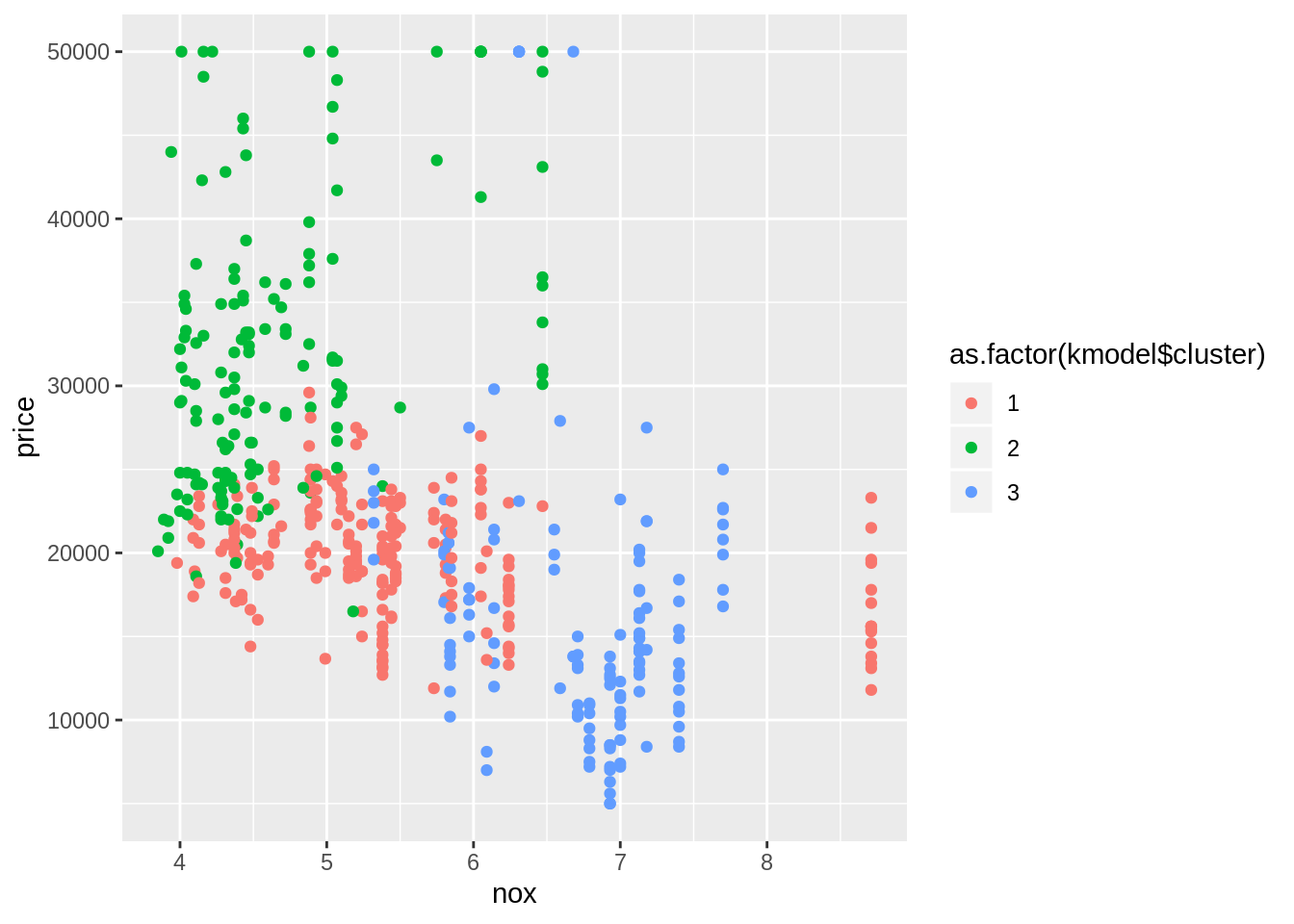
ggplot(hprice2,aes(x=nox,y=price,color=as.factor(kmodel$cluster))) + geom_point()
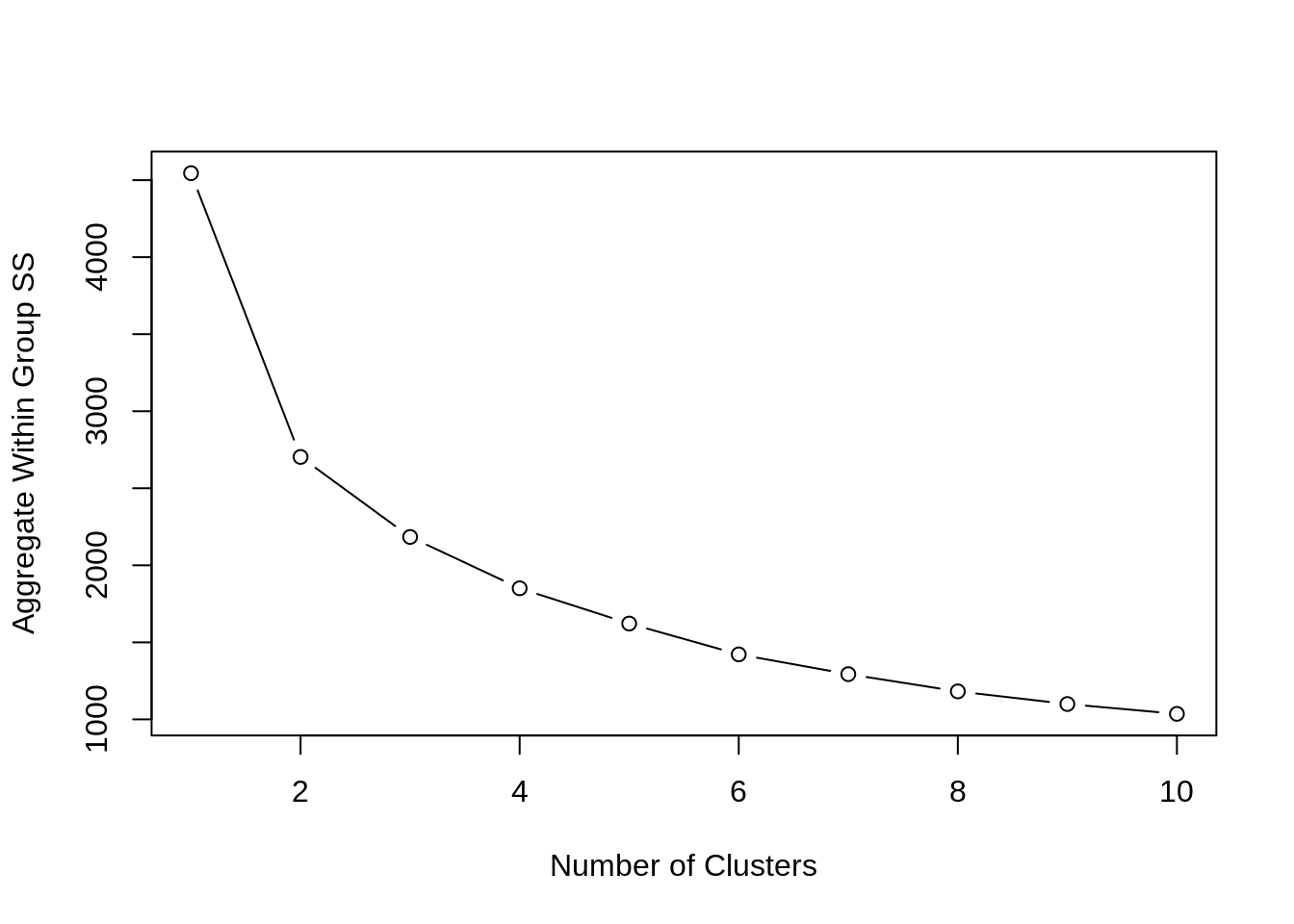
Within group sum of squares
## [1] 2183.669
kmeans.wss(scale(hprice2))
##  [1] 4545.000 2703.341 2183.948 1850.740 1621.996 1421.727 1293.463
##  [8] 1181.626 1099.631 1035.744
plot.wss(kmeans.wss(scale(hprice2)))
eratio <- function(wss) { # USE MINUS 1 FOR PCA
  # Creates the eigenvalue ratio estimator for the number of clusters
  n <- NROW(wss)
  dss <- -diff(wss) # Create differences in wss (eigenvalues)
  dss <- c(wss[1]/log(n),dss) # Assign a zero case
  erat <- dss[1:(n-1)]/dss[2:n] # Build the eigenvalue ratio statistic
  gss <- log(1+dss/wss) # Create growth rates
  grat <- gss[1:(n-1)]/gss[2:n] # Calucluate the growth rate statistic
  return(c(which.max(erat),which.max(grat))) # Find the maximum number for each estimator
}
eratio(kmeans.wss(scale(hprice2)))
## [1] 2 2
Hierarchical clustering algorithm
# Model dendrogram
model <- hclust(dist(scale(hprice2)))
summary(cutree(model,k=2))
##    Min. 1st Qu.  Median    Mean 3rd Qu.    Max.
##   1.000   1.000   1.000   1.073   1.000   2.000
hprice2[,lapply(.SD,mean),by=cutree(model,k=3)]
##    cutree     price     crime      nox    rooms     dist    radial
## 1:      1 23474.439  1.929987 5.448635 6.349190 3.968465  8.409382
## 2:      2 10503.294 20.348294 6.833824 5.392647 1.611471 24.000000
## 3:      3  8066.667 76.810333 6.810000 6.203333 1.550000 24.000000
##     proptax  stratio  lowstat
## 1: 38.79019 18.32196 11.65881
## 2: 66.60000 20.20000 26.41647
## 3: 66.60000 20.20000 20.27000
plot.wss(hclust.wss(data.table(scale(hprice2))))
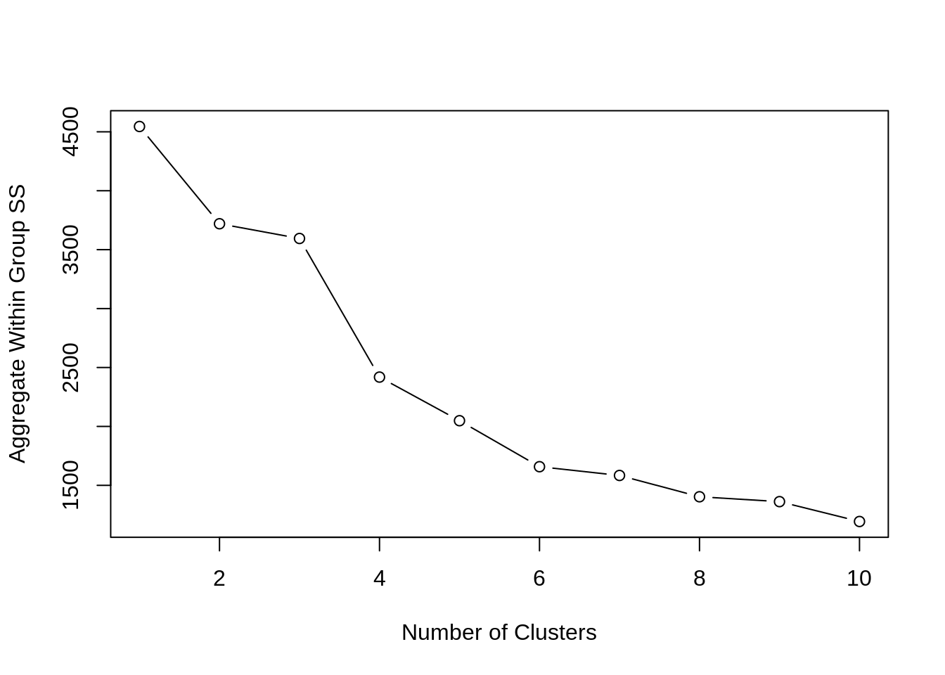
eratio(hclust.wss(data.table(scale(hprice2))))
## [1] 2 2
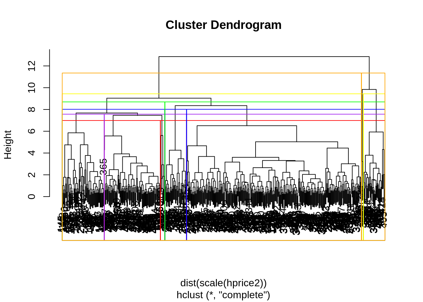
Dendrogram
plot(model)
rect.hclust(model,k=7,border="red")
rect.hclust(model,k=6,border="purple")
rect.hclust(model,k=5,border="blue")
rect.hclust(model,k=4,border="green")
rect.hclust(model,k=3,border="yellow")
rect.hclust(model,k=2,border="orange")
Applying clustering
set.seed(90210)
hprice2$kmean <- kmeans(scale(hprice2),centers=2,nstart=10)$cluster
hprice2$hier <- cutree(hclust(dist(data.table(scale(hprice2)))),k=4)
table(hprice2$hier,hprice2$kmean) # Two-way table to see relationship
##
##       1   2
##   1 235   0
##   2 111 123
##   3   0  34
##   4   0   3
# k-means clustering models
# Pooled:
summary(lm(log(price)~log(nox)+rooms+stratio,data=hprice2))
##
## Call:
## lm(formula = log(price) ~ log(nox) + rooms + stratio, data = hprice2)
##
## Residuals:
##      Min       1Q   Median       3Q      Max
## -1.02357 -0.13576  0.02406  0.13258  1.40083
##
## Coefficients:
##              Estimate Std. Error t value Pr(>|t|)
## (Intercept) 10.359458   0.219069  47.288   <2e-16 ***
## log(nox)    -0.645329   0.062580 -10.312   <2e-16 ***
## rooms        0.256727   0.018677  13.746   <2e-16 ***
## stratio     -0.050873   0.005926  -8.585   <2e-16 ***
## ---
## Signif. codes:  0 '***' 0.001 '**' 0.01 '*' 0.05 '.' 0.1 ' ' 1
##
## Residual standard error: 0.2673 on 502 degrees of freedom
## Multiple R-squared:  0.576,  Adjusted R-squared:  0.5734
## F-statistic: 227.3 on 3 and 502 DF,  p-value: < 2.2e-16
# Within:
summary(lm(log(price)~as.factor(kmean)+log(nox)+rooms+stratio-1,data=hprice2))
##
## Call:
## lm(formula = log(price) ~ as.factor(kmean) + log(nox) + rooms +
##     stratio - 1, data = hprice2)
##
## Residuals:
##      Min       1Q   Median       3Q      Max
## -0.98976 -0.12245  0.00579  0.11441  1.45933
##
## Coefficients:
##                    Estimate Std. Error t value Pr(>|t|)
## as.factor(kmean)1  9.787719   0.254704  38.428  < 2e-16 ***
## as.factor(kmean)2  9.611210   0.279304  34.411  < 2e-16 ***
## log(nox)          -0.357760   0.091938  -3.891 0.000113 ***
## rooms              0.253544   0.018389  13.788  < 2e-16 ***
## stratio           -0.042169   0.006185  -6.818 2.67e-11 ***
## ---
## Signif. codes:  0 '***' 0.001 '**' 0.01 '*' 0.05 '.' 0.1 ' ' 1
##
## Residual standard error: 0.2629 on 501 degrees of freedom
## Multiple R-squared:  0.9993, Adjusted R-squared:  0.9993
## F-statistic: 1.448e+05 on 5 and 501 DF,  p-value: < 2.2e-16
# hierarchical clustering models
# Pooled:
summary(lm(log(price)~log(nox)+rooms+stratio,data=hprice2))
##
## Call:
## lm(formula = log(price) ~ log(nox) + rooms + stratio, data = hprice2)
##
## Residuals:
##      Min       1Q   Median       3Q      Max
## -1.02357 -0.13576  0.02406  0.13258  1.40083
##
## Coefficients:
##              Estimate Std. Error t value Pr(>|t|)
## (Intercept) 10.359458   0.219069  47.288   <2e-16 ***
## log(nox)    -0.645329   0.062580 -10.312   <2e-16 ***
## rooms        0.256727   0.018677  13.746   <2e-16 ***
## stratio     -0.050873   0.005926  -8.585   <2e-16 ***
## ---
## Signif. codes:  0 '***' 0.001 '**' 0.01 '*' 0.05 '.' 0.1 ' ' 1
##
## Residual standard error: 0.2673 on 502 degrees of freedom
## Multiple R-squared:  0.576,  Adjusted R-squared:  0.5734
## F-statistic: 227.3 on 3 and 502 DF,  p-value: < 2.2e-16
# Within:
summary(lm(log(price)~as.factor(hier)+log(nox)+rooms+stratio,data=hprice2))
##
## Call:
## lm(formula = log(price) ~ as.factor(hier) + log(nox) + rooms +
##     stratio, data = hprice2)
##
## Residuals:
##      Min       1Q   Median       3Q      Max
## -0.95937 -0.13982  0.01699  0.11803  1.30258
##
## Coefficients:
##                  Estimate Std. Error t value Pr(>|t|)
## (Intercept)      10.10932    0.22968  44.015  < 2e-16 ***
## as.factor(hier)2 -0.06596    0.04174  -1.580    0.115
## as.factor(hier)3 -0.42904    0.06856  -6.258 8.41e-10 ***
## as.factor(hier)4 -0.87087    0.15113  -5.762 1.45e-08 ***
## log(nox)         -0.42487    0.08843  -4.805 2.05e-06 ***
## rooms             0.21876    0.01895  11.542  < 2e-16 ***
## stratio          -0.04112    0.00634  -6.487 2.11e-10 ***
## ---
## Signif. codes:  0 '***' 0.001 '**' 0.01 '*' 0.05 '.' 0.1 ' ' 1
##
## Residual standard error: 0.2484 on 499 degrees of freedom
## Multiple R-squared:  0.6361, Adjusted R-squared:  0.6317
## F-statistic: 145.4 on 6 and 499 DF,  p-value: < 2.2e-16