3.1 Derivation and foundations
3.1.1 Derivation
3.1.1.1 Problem specification
3.1.1.2 Solution
3.1.1.3 Implementation
Suppose that we want to fit a linear model: \[y_i=\beta_0+\beta_1x_i+e_i\] For instance, in the bwght data we might want to relate birthweight to cigarette smoking or \[\text{bwght}_i=\beta_0+\beta_1\text{cigs}_i+e_i\] The fitted model would then be: \[\text{bwght}_i=\hat\beta_0+\hat\beta_1\text{cigs}_i+\hat e_i\] \[\text{bwght}_i=119.77-0.5138\text{cigs}_i+\hat e_i\] This means that for every 1 cigarette smoked by the mother per day during pregnancy is associated with a 0.514 oz decrease in the expected birthweight of the child.
modela <- lm(bwght~cigs,data=bwght)
modela
##
## Call:
## lm(formula = bwght ~ cigs, data = bwght)
##
## Coefficients:
## (Intercept) cigs
## 119.7719 -0.5138If we want to get summary statistics for the model (hypothesis testing, R-squared, etc.), we just call:
summary(modela)##
## Call:
## lm(formula = bwght ~ cigs, data = bwght)
##
## Residuals:
## Min 1Q Median 3Q Max
## -96.772 -11.772 0.297 13.228 151.228
##
## Coefficients:
## Estimate Std. Error t value Pr(>|t|)
## (Intercept) 119.77190 0.57234 209.267 < 2e-16 ***
## cigs -0.51377 0.09049 -5.678 1.66e-08 ***
## ---
## Signif. codes: 0 '***' 0.001 '**' 0.01 '*' 0.05 '.' 0.1 ' ' 1
##
## Residual standard error: 20.13 on 1386 degrees of freedom
## Multiple R-squared: 0.02273, Adjusted R-squared: 0.02202
## F-statistic: 32.24 on 1 and 1386 DF, p-value: 1.662e-08To plot linear models, we are again going to use the ggplot2 package (Wickham et al. 2018). This plot is the same as the ones we created before just with a different data set:
plot4_basic <- ggplot(bwght,aes(x=cigs,y=bwght)) + geom_point()
plot4_basic <- plot4_basic + scale_x_continuous(name="Cigarettes smoked during pregnancy per day") + scale_y_continuous(name="Birthweight (oz)")
plot4_basic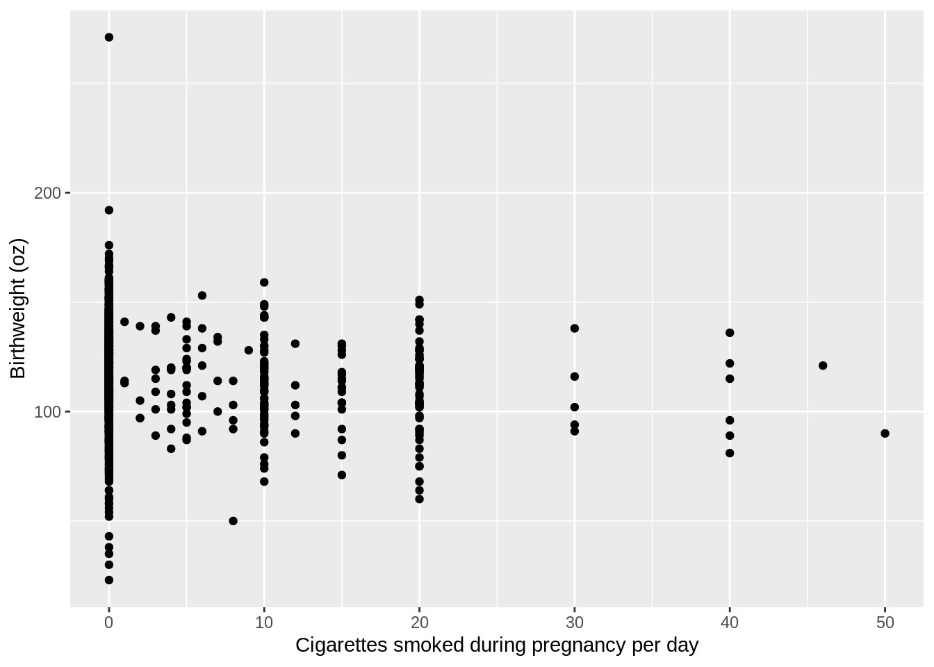
Now we need to add the line from our linear model, modela. we are going to use the geom_line() function to add the line. We have to specify the y values of the line associated with the x points of our data. To find these y values, we just need to use the predict function from before:
plot4_ols <- plot4_basic + geom_line(aes(y=predict(modela)),color="red",size=2)
plot4_ols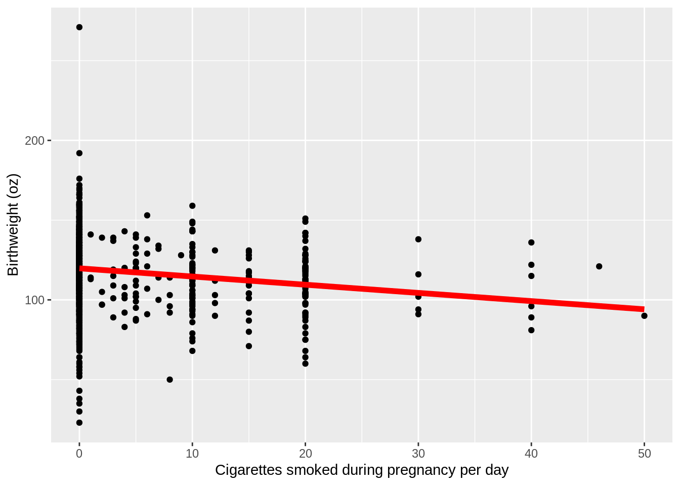
The broom package (Robinson and Hayes 2018) has various functions which standardize output from models. After installing the broom package it can be read into memory with:
library(broom)The first and most import broom command is tidy which takes the summary output from a linear model (or other models later) and formats the table of coefficients into a clean format:
tidy(modela)| term | estimate | std.error | statistic | p.value |
|---|---|---|---|---|
| (Intercept) | 119.7719004 | 0.5723407 | 209.266802 | 0 |
| cigs | -0.5137721 | 0.0904909 | -5.677609 | 0 |
The summary output also produces some various statistis about the model such as the \(R^2\) value. If you want a simple format for those results, you can use the glance function on the model:
glance(modela)| Variables | Values |
|---|---|
| r.squared | 2.272910e-02 |
| adj.r.squared | 2.202400e-02 |
| sigma | 2.012858e+01 |
| statistic | 3.223524e+01 |
| p.value | 0.000000e+00 |
| df | 2.000000e+00 |
| logLik | -6.135457e+03 |
| AIC | 1.227691e+04 |
| BIC | 1.229262e+04 |
| deviance | 5.615513e+05 |
| df.residual | 1.386000e+03 |
This also gives other statistics such as the AIC and BIC which are useful for model selection. Augment gives the original data with the residuals and fitted values:
summary(augment(modela))## bwght cigs .fitted .se.fit
## Min. : 23.0 Min. : 0.000 Min. : 94.08 Min. :0.5403
## 1st Qu.:107.0 1st Qu.: 0.000 1st Qu.:119.77 1st Qu.:0.5723
## Median :120.0 Median : 0.000 Median :119.77 Median :0.5723
## Mean :118.7 Mean : 2.087 Mean :118.70 Mean :0.6741
## 3rd Qu.:132.0 3rd Qu.: 0.000 3rd Qu.:119.77 3rd Qu.:0.5723
## Max. :271.0 Max. :50.000 Max. :119.77 Max. :4.3692
## .resid .hat .sigma .cooksd
## Min. :-96.772 Min. :0.0007206 Min. :19.72 Min. :5.000e-08
## 1st Qu.:-11.772 1st Qu.:0.0008085 1st Qu.:20.13 1st Qu.:3.877e-05
## Median : 0.297 Median :0.0008085 Median :20.13 Median :1.771e-04
## Mean : 0.000 Mean :0.0014409 Mean :20.13 Mean :7.080e-04
## 3rd Qu.: 13.228 3rd Qu.:0.0008085 3rd Qu.:20.14 3rd Qu.:5.403e-04
## Max. :151.228 Max. :0.0471172 Max. :20.14 Max. :5.279e-02
## .std.resid
## Min. :-4.809631
## 1st Qu.:-0.585072
## Median : 0.014764
## Mean : 0.000038
## 3rd Qu.: 0.657446
## Max. : 7.5161433.1.1.4 R-squared
3.1.2 Conditional expectation and predictions
3.1.2.1 Conditional expectation
3.1.2.2 Linear models
3.1.2.3 Predictions and residuals
To make predictions based on a model, e.g., \[\hat{bwght}=\hat\beta_0+\hat\beta_1cigs\], we can use the predict() function (e.g., predict(modela)). Because we only specify the model with the predictions, R doesn’t know what x values we want to use. So in this case it defaults to using the original x variables. This gives us the so-called fitted values. of the model:
summary(predict(modela))## Min. 1st Qu. Median Mean 3rd Qu. Max.
## 94.08 119.77 119.77 118.70 119.77 119.77If we want to make new predictions for two data points \(cigs=20\) and \(cigs=0\), we can add these x-values to the predict function:
predict(modela,data.table(cigs=c(20,0)))## 1 2
## 109.4965 119.77193.1.3 Matrix algebra representation
3.1.3.1 Multiple regression
3.1.3.2 Derivation
3.1.3.3 Implementation
3.1.3.4 Multiple regression with LM
3.1.4 Special models
3.1.4.1 Binary independent variables
Suppose we want to run a multiple regression: \[\text{bwght}_i=\beta_0+\beta_1 \text{cigs}_i+\beta_2 \text{faminc}_i + \text{male}_i+e_i\] To run this model, we simply enter:
modelb <- lm(bwght~cigs+faminc+male,data=bwght)
summary(modelb)
##
## Call:
## lm(formula = bwght ~ cigs + faminc + male, data = bwght)
##
## Residuals:
## Min 1Q Median 3Q Max
## -97.521 -11.577 0.994 13.194 151.655
##
## Coefficients:
## Estimate Std. Error t value Pr(>|t|)
## (Intercept) 115.22771 1.20788 95.397 < 2e-16 ***
## cigs -0.46105 0.09134 -5.048 5.07e-07 ***
## faminc 0.09688 0.02915 3.324 0.00091 ***
## male 3.11397 1.07640 2.893 0.00388 **
## ---
## Signif. codes: 0 '***' 0.001 '**' 0.01 '*' 0.05 '.' 0.1 ' ' 1
##
## Residual standard error: 20.01 on 1384 degrees of freedom
## Multiple R-squared: 0.03564, Adjusted R-squared: 0.03355
## F-statistic: 17.05 on 3 and 1384 DF, p-value: 7.105e-11This notation inside the lm command is called formula notation. A helpful guide on formula notation in R is available from the Booth School of Business.
Here, a \(1\) cigarette increase is associated with a \(-0.461\) decrease in \(oz\) of birthweight, but now we are controlling for family income and whether or not the child was male. To understand why we’re saying this consider two predictions. One child is a boy who is born with a mother who smokes \(20\) cigarettes per day has a family income of \(\$30,000\). The other child is also a boy whose mother smokes \(0\) cigarettes per day and also has a family income of \(\$30,000\). Clearly we are keeping family income and child sex constant. In this case the difference between the two predicted birthweights would be: \[\hat y_{20}-\hat y_{0}= 20\hat\beta_1+30\hat\beta_2+\hat\beta_3-0\hat\beta_1-30\hat\beta_2-\hat\beta_3\] \[\hat y_{20}-\hat y_{0}= 20\hat\beta_1=-9.22oz\] which is \(20\) times the estimated \(\beta_1\) value because this is a difference of \(20\) cigarettes per day.
In this linear model, we could also consider an interpretation for the \(\beta_3\) coefficient. If a child is male, then \(\text{male}_i=1\) otherwise \(\text{male}_i=0\). This means that if the child is male, we expect the birthweight to increase by \(\hat\beta_3=3.11oz\) controlling for cigarette smoking and family income. This is how we interpret models with binary or “dummy” variables.
3.1.4.2 Quadratics and polynomial functions
To perform a quadratic regression such as: \[\text{bwght}_i=\beta_0+\beta_1\text{cigs}_i+\beta_2\text{cigs}_i^2+e_i\] we have to use the I() function in R. I() tells R to ignore the special formula notation and do literally what commands we input. Here we are taking the square. So the I(cigs^2) says add \(\text{cigs}^2\) to the linear model:
modelc <- lm(bwght~cigs+I(cigs^2),data=bwght)
summary(modelc)
##
## Call:
## lm(formula = bwght ~ cigs + I(cigs^2), data = bwght)
##
## Residuals:
## Min 1Q Median 3Q Max
## -96.949 -11.949 1.051 13.051 151.051
##
## Coefficients:
## Estimate Std. Error t value Pr(>|t|)
## (Intercept) 119.949119 0.579843 206.865 < 2e-16 ***
## cigs -0.858407 0.207398 -4.139 3.7e-05 ***
## I(cigs^2) 0.013551 0.007339 1.846 0.065 .
## ---
## Signif. codes: 0 '***' 0.001 '**' 0.01 '*' 0.05 '.' 0.1 ' ' 1
##
## Residual standard error: 20.11 on 1385 degrees of freedom
## Multiple R-squared: 0.02513, Adjusted R-squared: 0.02372
## F-statistic: 17.85 on 2 and 1385 DF, p-value: 2.218e-083.1.4.3 Interactions
To include interactions between two variables, you can use the formula notaion for interactions which is a:b to interact (essentially multiply) a and b and include the result in the model:
bwght$smokes <- as.numeric(bwght$cigs>0)
modele <- lm(bwght~smokes+faminc+male+white+smokes:faminc+smokes:male+smokes:white,data=bwght)
summary(modele)
##
## Call:
## lm(formula = bwght ~ smokes + faminc + male + white + smokes:faminc +
## smokes:male + smokes:white, data = bwght)
##
## Residuals:
## Min 1Q Median 3Q Max
## -93.340 -11.681 0.563 12.981 150.882
##
## Coefficients:
## Estimate Std. Error t value Pr(>|t|)
## (Intercept) 112.02091 1.54585 72.465 < 2e-16 ***
## smokes -5.54028 3.83280 -1.445 0.14855
## faminc 0.04112 0.03225 1.275 0.20255
## male 3.39415 1.16286 2.919 0.00357 **
## white 6.34911 1.48836 4.266 2.13e-05 ***
## smokes:faminc 0.12468 0.10066 1.239 0.21569
## smokes:male -2.85699 3.00414 -0.951 0.34176
## smokes:white -5.13610 3.73596 -1.375 0.16942
## ---
## Signif. codes: 0 '***' 0.001 '**' 0.01 '*' 0.05 '.' 0.1 ' ' 1
##
## Residual standard error: 19.88 on 1380 degrees of freedom
## Multiple R-squared: 0.05043, Adjusted R-squared: 0.04561
## F-statistic: 10.47 on 7 and 1380 DF, p-value: 7.211e-13Here, I have interacted a dummy for smoking behavior with faminc, male, white. To include all the pairwise interactions we can enter:
bwght$smokes <- as.numeric(bwght$cigs>0)
modelf <- lm(bwght~(smokes+faminc+male+white)^2,data=bwght)
summary(modelf)
##
## Call:
## lm(formula = bwght ~ (smokes + faminc + male + white)^2, data = bwght)
##
## Residuals:
## Min 1Q Median 3Q Max
## -93.463 -11.706 0.626 13.163 150.943
##
## Coefficients:
## Estimate Std. Error t value Pr(>|t|)
## (Intercept) 113.08465 2.44118 46.324 <2e-16 ***
## smokes -6.05461 3.88408 -1.559 0.1193
## faminc -0.02513 0.08240 -0.305 0.7604
## male 2.92238 2.65627 1.100 0.2714
## white 5.87552 2.80561 2.094 0.0364 *
## smokes:faminc 0.12521 0.10109 1.239 0.2157
## smokes:male -2.37318 3.06905 -0.773 0.4395
## smokes:white -4.75201 3.79282 -1.253 0.2105
## faminc:male 0.04539 0.06128 0.741 0.4590
## faminc:white 0.05094 0.08315 0.613 0.5402
## male:white -1.16949 2.74399 -0.426 0.6700
## ---
## Signif. codes: 0 '***' 0.001 '**' 0.01 '*' 0.05 '.' 0.1 ' ' 1
##
## Residual standard error: 19.9 on 1377 degrees of freedom
## Multiple R-squared: 0.05112, Adjusted R-squared: 0.04423
## F-statistic: 7.418 on 10 and 1377 DF, p-value: 1.482e-11Incidentally this is why we have to use the I() function to create quadratics. In formula notation a^b is used for adding interactions, not making things quadratic. Be careful about your notation here.
3.1.4.4 Log-linear specifications
If we want to take the natural logarithm of one of the variables, we simply surround that variable with the log() function:
modeld <- lm(log(bwght)~cigs+faminc,data=bwght)
summary(modeld)
##
## Call:
## lm(formula = log(bwght) ~ cigs + faminc, data = bwght)
##
## Residuals:
## Min 1Q Median 3Q Max
## -1.62745 -0.08761 0.02148 0.12155 0.82230
##
## Coefficients:
## Estimate Std. Error t value Pr(>|t|)
## (Intercept) 4.7439566 0.0098431 481.958 < 2e-16 ***
## cigs -0.0040326 0.0008593 -4.693 2.96e-06 ***
## faminc 0.0008437 0.0002739 3.081 0.00211 **
## ---
## Signif. codes: 0 '***' 0.001 '**' 0.01 '*' 0.05 '.' 0.1 ' ' 1
##
## Residual standard error: 0.1883 on 1385 degrees of freedom
## Multiple R-squared: 0.02646, Adjusted R-squared: 0.02505
## F-statistic: 18.82 on 2 and 1385 DF, p-value: 8.608e-09References
Wickham, Hadley, Winston Chang, Lionel Henry, Thomas Lin Pedersen, Kohske Takahashi, Claus Wilke, and Kara Woo. 2018. Ggplot2: Create Elegant Data Visualisations Using the Grammar of Graphics. https://CRAN.R-project.org/package=ggplot2.
Robinson, David, and Alex Hayes. 2018. Broom: Convert Statistical Analysis Objects into Tidy Tibbles. https://CRAN.R-project.org/package=broom.