5.3 Coding guide

5.3.1 Preparing the data

For most time series analysis, we are going to be using a few different packages: forecast, tseries, TSA, and vars. That said, it’s a good idea to only use the library command on forecast. The reason for this is that the other packages have some functions that can override the built-in R versions and cause breakages. The data we are going to be working on here is the minwage table from the Wooldridge database.

library(forecast)
n <- nrow(minwage)
minwage$emp <- minwage$emp232
minwage$wage <- minwage$wage232
minwage <- minwage[,.(index,cpi,emp,wage)]

5.3.2 Stationarity testing

To test for stationarity, we are going to use the Krawatski-Phillips-Schmidt-Shin (KPSS) test. There are other tests for stationarity, but the KPSS test is the easiest to use and probabily the easies to interpret. The null hypothesis for the test is that the series is either level or trend stationary (depending on what you set in the function). The althernative is that the series is not level or trend stationary (depending on your settings). To perform the test, we are going to use the tseries package:

tseries::kpss.test(minwage$emp,null="Level")

## Warning in tseries::kpss.test(minwage$emp, null = "Level"): p-value smaller
## than printed p-value

## 
##  KPSS Test for Level Stationarity
## 
## data:  minwage$emp
## KPSS Level = 2.0421, Truncation lag parameter = 6, p-value = 0.01

The two places to look for information from a KPSS test are the \(p\)-value and the function call (i.e., what you put into the function). Above we tested if the emp series was “level” stationary (without differencing because we didn’t use the diff function). The result of the test is that we reject the null hypothesis even at the \(1\%\) level. The function may give some warning messages, it is safe to ignore those (the reason is that the \(p\)-value is technically an approximation which suffers below \(1\%\) and above \(10\%\)). The result from all this is that we know emp is not level stationry. Now we will test it for trend stationarity:

tseries::kpss.test(minwage$emp,null="Trend")

## Warning in tseries::kpss.test(minwage$emp, null = "Trend"): p-value smaller
## than printed p-value

## 
##  KPSS Test for Trend Stationarity
## 
## data:  minwage$emp
## KPSS Trend = 2.0419, Truncation lag parameter = 6, p-value = 0.01

Here we also see that employment is not trend stationary. Since we know employment is neither level or trend stationary, try taking differences and testing again:

tseries::kpss.test(diff(minwage$emp),null="Level")

## 
##  KPSS Test for Level Stationarity
## 
## data:  diff(minwage$emp)
## KPSS Level = 0.60423, Truncation lag parameter = 6, p-value =
## 0.02225

Now we also see that employmnent is not level stationary after first-differencing, so we test for trend stationarity:

tseries::kpss.test(diff(minwage$emp),null="Trend")

## Warning in tseries::kpss.test(diff(minwage$emp), null = "Trend"): p-value
## greater than printed p-value

## 
##  KPSS Test for Trend Stationarity
## 
## data:  diff(minwage$emp)
## KPSS Trend = 0.055668, Truncation lag parameter = 6, p-value = 0.1

Finally, now that the \(p\)-value is greater than \(5\%\), we know that employment is trend stationary after taking first-differences. Note that it is possible to put this into a function with a loop to save yourself time in the future. This is left as an exercise because it is a useful learning experience. You might want to learn about the suppresssWarnings function to keep R from giving a bunch of warnings here.

5.3.3 Time series plots

Basic time series plots can be obtained by using the ts.plot function:

ts.plot(minwage$cpi) # Data is monthly from 1950 to 2001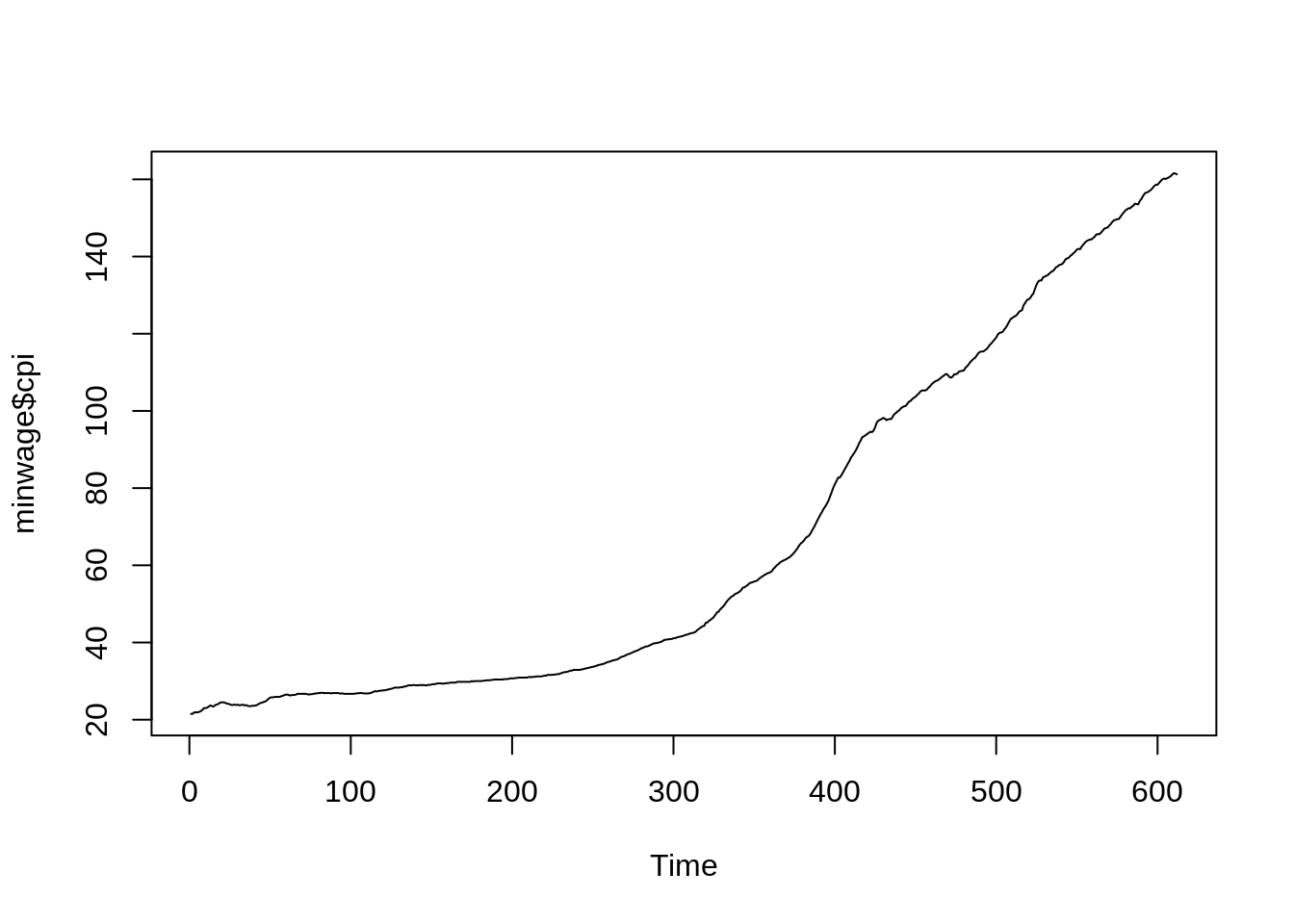

These plots don’t look very good, so instead we are going to use ggplot:

minwage$date <- seq(1950,2001-1/12,1/12)
ggplot(minwage,aes(x=date,y=wage))+geom_line()+
  scale_x_continuous('Year')+
  scale_y_continuous('Hourly wage')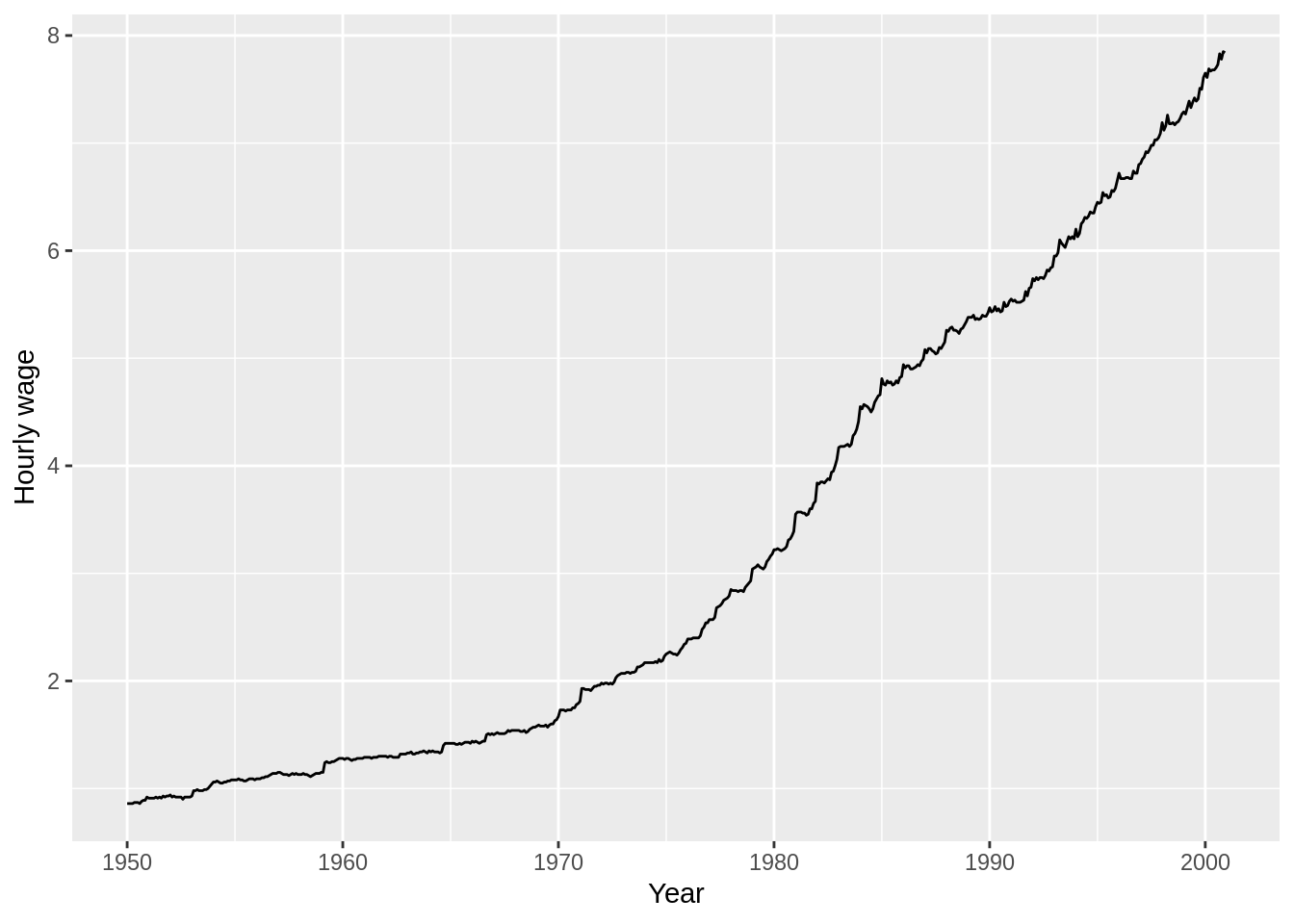

ggplot(minwage,aes(x=date,y=emp))+geom_line()+
  scale_x_continuous('Year')+
  scale_y_continuous('Total employment')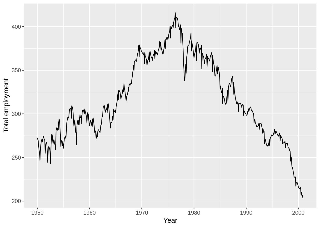

We can get similar autocorrelation function and partial autocorrelation function plots using the acf and pacf commands:

acf(diff(log(minwage$wage)))

I prefer to use the ggtsdisplay from the forecast package. Note that it’s critical to use the stationary-transformed process when plotting the ACF and PACF.

ggtsdisplay(diff(log(minwage$wag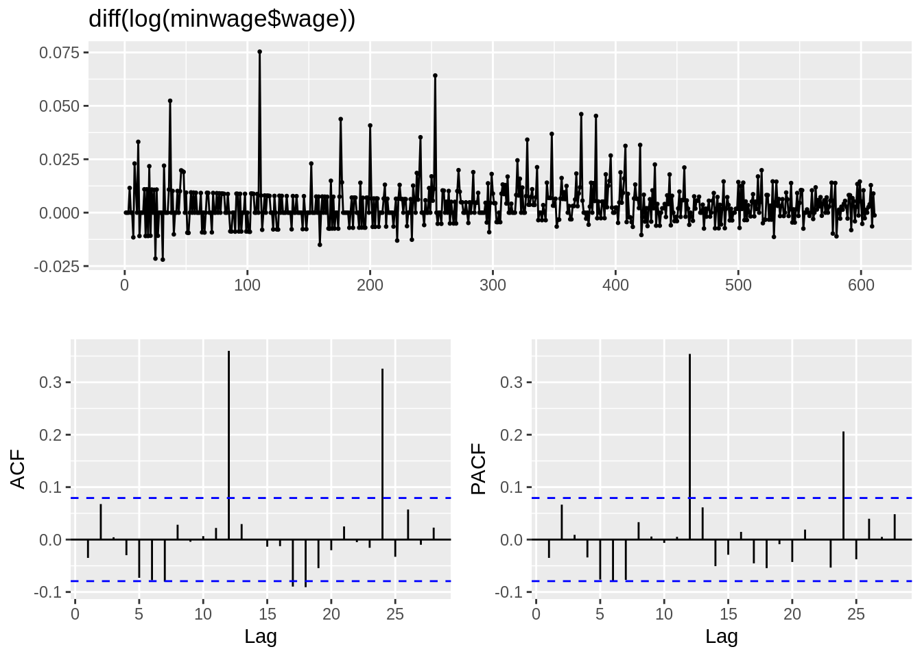e)))

The TSA package has a function for the periodogram to see seasonality in the data. It is also important to use the stationary-transformed data here too.

TSA::periodogram(diff(log(minwage$wage)))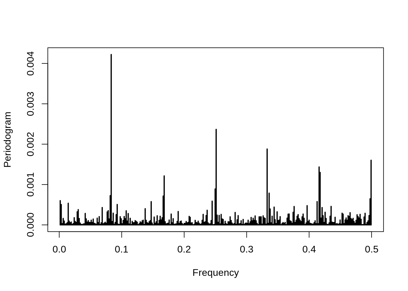

5.3.4 Regression with time series

model1 <- lm(log(emp)~log(wage)+index,data=minwage)
summary(model1)

## 
## Call:
## lm(formula = log(emp) ~ log(wage) + index, data = minwage)
## 
## Residuals:
##      Min       1Q   Median       3Q      Max 
## -0.43853 -0.10921 -0.01709  0.12802  0.25048 
## 
## Coefficients:
##               Estimate Std. Error t value Pr(>|t|)    
## (Intercept)  5.6626481  0.0210231 269.354  < 2e-16 ***
## log(wage)   -0.3671217  0.0636350  -5.769 1.27e-08 ***
## index        0.0013847  0.0002532   5.468 6.64e-08 ***
## ---
## Signif. codes:  0 '***' 0.001 '**' 0.01 '*' 0.05 '.' 0.1 ' ' 1
## 
## Residual standard error: 0.1473 on 609 degrees of freedom
## Multiple R-squared:  0.05698,    Adjusted R-squared:  0.05388 
## F-statistic:  18.4 on 2 and 609 DF,  p-value: 1.745e-08

model2 <- lm(diff(log(emp))~diff(log(wage))+index[2:n],data=minwage)
summary(model2)

## 
## Call:
## lm(formula = diff(log(emp)) ~ diff(log(wage)) + index[2:n], data = minwage)
## 
## Residuals:
##       Min        1Q    Median        3Q       Max 
## -0.072426 -0.007725  0.000590  0.008394  0.080283 
## 
## Coefficients:
##                   Estimate Std. Error t value Pr(>|t|)  
## (Intercept)      2.496e-03  1.530e-03   1.631   0.1034  
## diff(log(wage)) -4.350e-02  8.017e-02  -0.543   0.5876  
## index[2:n]      -9.176e-06  4.264e-06  -2.152   0.0318 *
## ---
## Signif. codes:  0 '***' 0.001 '**' 0.01 '*' 0.05 '.' 0.1 ' ' 1
## 
## Residual standard error: 0.01859 on 608 degrees of freedom
## Multiple R-squared:  0.008085,   Adjusted R-squared:  0.004822 
## F-statistic: 2.478 on 2 and 608 DF,  p-value: 0.08476

lmtest::coeftest(model2,sandwich::NeweyWest)

## 
## t test of coefficients:
## 
##                    Estimate  Std. Error t value Pr(>|t|)  
## (Intercept)      2.4962e-03  1.4029e-03  1.7794  0.07567 .
## diff(log(wage)) -4.3501e-02  7.3725e-02 -0.5900  0.55538  
## index[2:n]      -9.1755e-06  3.6464e-06 -2.5163  0.01211 *
## ---
## Signif. codes:  0 '***' 0.001 '**' 0.01 '*' 0.05 '.' 0.1 ' ' 1

5.3.5 ARIMA models

To fit an ARIMA(p,d,q) model to the data simply enter:

model3 <- Arima(log(minwage$emp),c(4,1,4),include.drift=TRUE)
summary(model3)

## Series: log(minwage$emp) 
## ARIMA(4,1,4) with drift 
## 
## Coefficients:

## Warning in sqrt(diag(x$var.coef)): NaNs produced

##          ar1      ar2     ar3      ar4      ma1     ma2     ma3     ma4
##       0.4672  -0.4555  0.5427  -0.8051  -0.6975  0.6788  -0.668  0.8994
## s.e.  0.0239      NaN  0.0335   0.0357      NaN     NaN     NaN  0.0213
##        drift
##       -5e-04
## s.e.   6e-04
## 
## sigma^2 estimated as 0.0002623:  log likelihood=1655.23
## AIC=-3290.45   AICc=-3290.09   BIC=-3246.3
## 
## Training set error measures:
##                        ME       RMSE        MAE         MPE      MAPE
## Training set 5.081071e-05 0.01606285 0.01184991 2.80847e-05 0.2068586
##                   MASE       ACF1
## Training set 0.9200793 0.03590587

Here, I have fit an ARIMA(4,1,4) model with a drift for the wage. I chose d=1 and included the drift because the series was trend stationary after first-differencing. The AIC and BIC functions can be used to find the optimal model. Here is the optimal model for the wage series:

model4 <- Arima(log(minwage$wage),c(12,1,12))

Now we forecast future wages in this sector using the forecast package.

steps <- 60
future <- forecast(model4,h=steps)
autoplot(future)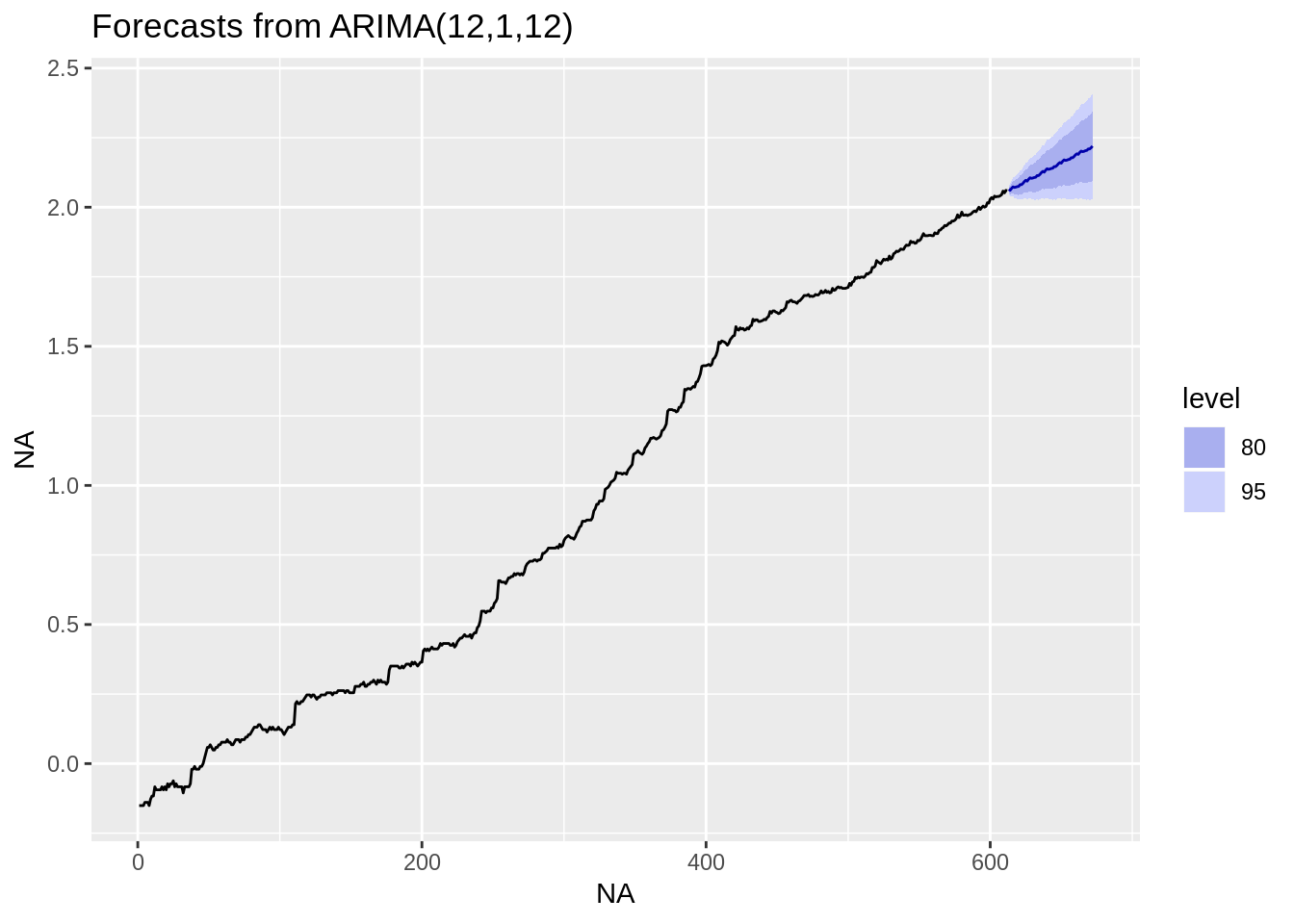

This plot shows the future predictions at the \(80\%\) and \(95\%\) confidence levels. To zoom in on the unknown area:

autoplot(future,xlim=c(n-steps,n+steps),ylim=c(1.5,2.5))

## Scale for 'x' is already present. Adding another scale for 'x', which
## will replace the existing scale.

## Warning: Removed 551 rows containing missing values (geom_path).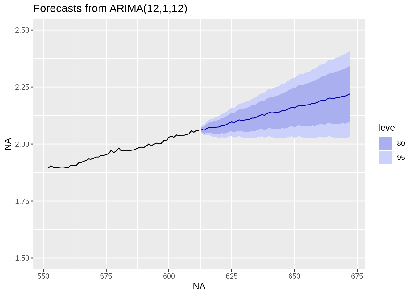

We know there is serious year-to-year seasonality in the data, so we might want to fit a seasonal ARIMA to the model (with a 12-period lag because there are 12 months in a year):

model5 <- Arima(log(minwage$wage),c(0,1,2),
                seasonal=list(order=c(1,0,1),period=12))
summary(model5)

## Series: log(minwage$wage) 
## ARIMA(0,1,2)(1,0,1)[12] 
## 
## Coefficients:
##           ma1     ma2    sar1     sma1
##       -0.0425  0.0869  0.9568  -0.7695
## s.e.   0.0404  0.0417  0.0161   0.0421
## 
## sigma^2 estimated as 6.785e-05:  log likelihood=2063.08
## AIC=-4116.17   AICc=-4116.07   BIC=-4094.09
## 
## Training set error measures:
##                        ME       RMSE         MAE MPE MAPE      MASE
## Training set 0.0007223263 0.00820317 0.005222821 Inf  Inf 0.8225484
##                      ACF1
## Training set -0.005371024

This model has 2 normal moving average coefficients and an autoregressive and a moving average coefficient on the 12-month lag. Here is a visualization of our updated predictions:

steps <- 60
future2 <- forecast(model5,h=steps)
autoplot(future2,xlim=c(n-steps,n+steps),ylim=c(1.5,2.5))

## Scale for 'x' is already present. Adding another scale for 'x', which
## will replace the existing scale.

## Warning: Removed 551 rows containing missing values (geom_path).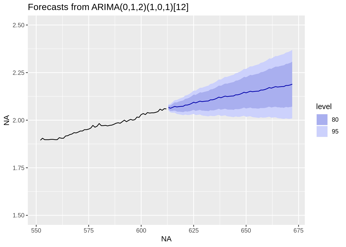

5.3.6 VAR models

xdata <- minwage[,.(diff(log(wage)),diff(log(emp)))]
model6 <- vars::VAR(xdata,p=1,type="both")
summary(model6)

## 
## VAR Estimation Results:
## ========================= 
## Endogenous variables: V1, V2 
## Deterministic variables: both 
## Sample size: 610 
## Log Likelihood: 3574.099 
## Roots of the characteristic polynomial:
## 0.2131 0.06997
## Call:
## vars::VAR(y = xdata, p = 1, type = "both")
## 
## 
## Estimation results for equation V1: 
## =================================== 
## V1 = V1.l1 + V2.l1 + const + trend 
## 
##         Estimate Std. Error t value Pr(>|t|)    
## V1.l1 -3.240e-02  4.030e-02  -0.804  0.42175    
## V2.l1  6.257e-02  2.038e-02   3.071  0.00223 ** 
## const  3.388e-03  7.730e-04   4.383 1.38e-05 ***
## trend  1.244e-06  2.156e-06   0.577  0.56407    
## ---
## Signif. codes:  0 '***' 0.001 '**' 0.01 '*' 0.05 '.' 0.1 ' ' 1
## 
## 
## Residual standard error: 0.00934 on 606 degrees of freedom
## Multiple R-Squared: 0.01668, Adjusted R-squared: 0.01181 
## F-statistic: 3.426 on 3 and 606 DF,  p-value: 0.01693 
## 
## 
## Estimation results for equation V2: 
## =================================== 
## V2 = V1.l1 + V2.l1 + const + trend 
## 
##         Estimate Std. Error t value Pr(>|t|)    
## V1.l1 -1.085e-01  7.769e-02  -1.396  0.16308    
## V2.l1 -2.507e-01  3.928e-02  -6.381  3.5e-10 ***
## const  3.277e-03  1.490e-03   2.199  0.02826 *  
## trend -1.135e-05  4.156e-06  -2.731  0.00649 ** 
## ---
## Signif. codes:  0 '***' 0.001 '**' 0.01 '*' 0.05 '.' 0.1 ' ' 1
## 
## 
## Residual standard error: 0.01801 on 606 degrees of freedom
## Multiple R-Squared: 0.0722,  Adjusted R-squared: 0.06761 
## F-statistic: 15.72 on 3 and 606 DF,  p-value: 7.414e-10 
## 
## 
## 
## Covariance matrix of residuals:
##           V1        V2
## V1 8.724e-05 1.298e-06
## V2 1.298e-06 3.242e-04
## 
## Correlation matrix of residuals:
##         V1      V2
## V1 1.00000 0.00772
## V2 0.00772 1.00000

c(AIC(model6),BIC(model6))

## [1] -7132.199 -7096.891

predict(model6,n.ahead=60)

## $V1
##              fcst       lower      upper         CI
##  [1,] 0.003883624 -0.01442296 0.02219021 0.01830659
##  [2,] 0.003880859 -0.01456742 0.02232914 0.01844828
##  [3,] 0.003805580 -0.01465361 0.02226477 0.01845919
##  [4,] 0.003827775 -0.01463202 0.02228757 0.01845979
##  [5,] 0.003823460 -0.01463636 0.02228328 0.01845982
##  [6,] 0.003825196 -0.01463463 0.02228502 0.01845983
##  [7,] 0.003825615 -0.01463421 0.02228544 0.01845983
##  [8,] 0.003826317 -0.01463351 0.02228614 0.01845983
##  [9,] 0.003826958 -0.01463287 0.02228678 0.01845983
## [10,] 0.003827611 -0.01463221 0.02228744 0.01845983
## [11,] 0.003828263 -0.01463156 0.02228809 0.01845983
## [12,] 0.003828914 -0.01463091 0.02228874 0.01845983
## [13,] 0.003829566 -0.01463026 0.02228939 0.01845983
## [14,] 0.003830217 -0.01462961 0.02229004 0.01845983
## [15,] 0.003830869 -0.01462896 0.02229069 0.01845983
## [16,] 0.003831521 -0.01462830 0.02229135 0.01845983
## [17,] 0.003832172 -0.01462765 0.02229200 0.01845983
## [18,] 0.003832824 -0.01462700 0.02229265 0.01845983
## [19,] 0.003833475 -0.01462635 0.02229330 0.01845983
## [20,] 0.003834127 -0.01462570 0.02229395 0.01845983
## [21,] 0.003834779 -0.01462505 0.02229460 0.01845983
## [22,] 0.003835430 -0.01462440 0.02229526 0.01845983
## [23,] 0.003836082 -0.01462374 0.02229591 0.01845983
## [24,] 0.003836734 -0.01462309 0.02229656 0.01845983
## [25,] 0.003837385 -0.01462244 0.02229721 0.01845983
## [26,] 0.003838037 -0.01462179 0.02229786 0.01845983
## [27,] 0.003838688 -0.01462114 0.02229851 0.01845983
## [28,] 0.003839340 -0.01462049 0.02229917 0.01845983
## [29,] 0.003839992 -0.01461983 0.02229982 0.01845983
## [30,] 0.003840643 -0.01461918 0.02230047 0.01845983
## [31,] 0.003841295 -0.01461853 0.02230112 0.01845983
## [32,] 0.003841946 -0.01461788 0.02230177 0.01845983
## [33,] 0.003842598 -0.01461723 0.02230242 0.01845983
## [34,] 0.003843250 -0.01461658 0.02230308 0.01845983
## [35,] 0.003843901 -0.01461592 0.02230373 0.01845983
## [36,] 0.003844553 -0.01461527 0.02230438 0.01845983
## [37,] 0.003845204 -0.01461462 0.02230503 0.01845983
## [38,] 0.003845856 -0.01461397 0.02230568 0.01845983
## [39,] 0.003846508 -0.01461332 0.02230633 0.01845983
## [40,] 0.003847159 -0.01461267 0.02230698 0.01845983
## [41,] 0.003847811 -0.01461201 0.02230764 0.01845983
## [42,] 0.003848462 -0.01461136 0.02230829 0.01845983
## [43,] 0.003849114 -0.01461071 0.02230894 0.01845983
## [44,] 0.003849766 -0.01461006 0.02230959 0.01845983
## [45,] 0.003850417 -0.01460941 0.02231024 0.01845983
## [46,] 0.003851069 -0.01460876 0.02231089 0.01845983
## [47,] 0.003851720 -0.01460810 0.02231155 0.01845983
## [48,] 0.003852372 -0.01460745 0.02231220 0.01845983
## [49,] 0.003853024 -0.01460680 0.02231285 0.01845983
## [50,] 0.003853675 -0.01460615 0.02231350 0.01845983
## [51,] 0.003854327 -0.01460550 0.02231415 0.01845983
## [52,] 0.003854979 -0.01460485 0.02231480 0.01845983
## [53,] 0.003855630 -0.01460420 0.02231546 0.01845983
## [54,] 0.003856282 -0.01460354 0.02231611 0.01845983
## [55,] 0.003856933 -0.01460289 0.02231676 0.01845983
## [56,] 0.003857585 -0.01460224 0.02231741 0.01845983
## [57,] 0.003858237 -0.01460159 0.02231806 0.01845983
## [58,] 0.003858888 -0.01460094 0.02231871 0.01845983
## [59,] 0.003859540 -0.01460029 0.02231937 0.01845983
## [60,] 0.003860191 -0.01459963 0.02232002 0.01845983
## 
## $V2
##               fcst       lower      upper         CI
##  [1,] -0.002302286 -0.03759421 0.03298964 0.03529192
##  [2,] -0.003526718 -0.03996829 0.03291486 0.03644157
##  [3,] -0.003230863 -0.03973063 0.03326890 0.03649977
##  [4,] -0.003308205 -0.03981072 0.03319431 0.03650252
##  [5,] -0.003302580 -0.03980522 0.03320006 0.03650264
##  [6,] -0.003314874 -0.03981752 0.03318777 0.03650265
##  [7,] -0.003323334 -0.03982598 0.03317931 0.03650265
##  [8,] -0.003332611 -0.03983526 0.03317004 0.03650265
##  [9,] -0.003341715 -0.03984436 0.03316093 0.03650265
## [10,] -0.003350855 -0.03985350 0.03315179 0.03650265
## [11,] -0.003359988 -0.03986264 0.03314266 0.03650265
## [12,] -0.003369122 -0.03987177 0.03313353 0.03650265
## [13,] -0.003378256 -0.03988090 0.03312439 0.03650265
## [14,] -0.003387390 -0.03989004 0.03311526 0.03650265
## [15,] -0.003396524 -0.03989917 0.03310612 0.03650265
## [16,] -0.003405658 -0.03990831 0.03309699 0.03650265
## [17,] -0.003414792 -0.03991744 0.03308786 0.03650265
## [18,] -0.003423926 -0.03992657 0.03307872 0.03650265
## [19,] -0.003433060 -0.03993571 0.03306959 0.03650265
## [20,] -0.003442193 -0.03994484 0.03306045 0.03650265
## [21,] -0.003451327 -0.03995398 0.03305132 0.03650265
## [22,] -0.003460461 -0.03996311 0.03304219 0.03650265
## [23,] -0.003469595 -0.03997224 0.03303305 0.03650265
## [24,] -0.003478729 -0.03998138 0.03302392 0.03650265
## [25,] -0.003487863 -0.03999051 0.03301478 0.03650265
## [26,] -0.003496997 -0.03999965 0.03300565 0.03650265
## [27,] -0.003506131 -0.04000878 0.03299652 0.03650265
## [28,] -0.003515265 -0.04001791 0.03298738 0.03650265
## [29,] -0.003524399 -0.04002705 0.03297825 0.03650265
## [30,] -0.003533533 -0.04003618 0.03296912 0.03650265
## [31,] -0.003542667 -0.04004531 0.03295998 0.03650265
## [32,] -0.003551801 -0.04005445 0.03295085 0.03650265
## [33,] -0.003560935 -0.04006358 0.03294171 0.03650265
## [34,] -0.003570069 -0.04007272 0.03293258 0.03650265
## [35,] -0.003579203 -0.04008185 0.03292345 0.03650265
## [36,] -0.003588337 -0.04009098 0.03291431 0.03650265
## [37,] -0.003597470 -0.04010012 0.03290518 0.03650265
## [38,] -0.003606604 -0.04010925 0.03289604 0.03650265
## [39,] -0.003615738 -0.04011839 0.03288691 0.03650265
## [40,] -0.003624872 -0.04012752 0.03287778 0.03650265
## [41,] -0.003634006 -0.04013665 0.03286864 0.03650265
## [42,] -0.003643140 -0.04014579 0.03285951 0.03650265
## [43,] -0.003652274 -0.04015492 0.03285037 0.03650265
## [44,] -0.003661408 -0.04016406 0.03284124 0.03650265
## [45,] -0.003670542 -0.04017319 0.03283211 0.03650265
## [46,] -0.003679676 -0.04018232 0.03282297 0.03650265
## [47,] -0.003688810 -0.04019146 0.03281384 0.03650265
## [48,] -0.003697944 -0.04020059 0.03280470 0.03650265
## [49,] -0.003707078 -0.04020973 0.03279557 0.03650265
## [50,] -0.003716212 -0.04021886 0.03278644 0.03650265
## [51,] -0.003725346 -0.04022799 0.03277730 0.03650265
## [52,] -0.003734480 -0.04023713 0.03276817 0.03650265
## [53,] -0.003743613 -0.04024626 0.03275903 0.03650265
## [54,] -0.003752747 -0.04025540 0.03274990 0.03650265
## [55,] -0.003761881 -0.04026453 0.03274077 0.03650265
## [56,] -0.003771015 -0.04027366 0.03273163 0.03650265
## [57,] -0.003780149 -0.04028280 0.03272250 0.03650265
## [58,] -0.003789283 -0.04029193 0.03271336 0.03650265
## [59,] -0.003798417 -0.04030107 0.03270423 0.03650265
## [60,] -0.003807551 -0.04031020 0.03269510 0.03650265