2.4 Statistics
2.4.1 Simulation studies
2.4.1.1 Synthetic data
Generating synthetic data is extremely easy in R. Let’s say we want to create \(100\) random uniform numbers with a minimum possible value of \(-2\) and a maximum of \(2\) and store them as a variable x. We just have to use the function runif (for random uniform):
x <- runif(100,min=-2,max=2)
summary(x)
## Min. 1st Qu. Median Mean 3rd Qu. Max.
## -1.99229 -0.69602 0.02020 0.08589 0.94485 1.99464You can also draw data from other distributions. The most common distribution we want to use is the normal distribution. You can draw random normal numbers with:
x <- rnorm(100,mean=5,sd=0.5)
c(mean(x),sd(x))
## [1] 4.9491458 0.5442711Here the population mean is \(5\) and the population standard deviation is \(0.5\). You can see that the sample statistics for the mean and standard deviation are different from the population numbers.
2.4.1.2 Setting seeds
When creating synthetic data it is important that we preserve reproducability. If I create random numbers on my computer, often I want you to be able to create the exact same random numbers on your computer. That way we can share code and get the same results. To make us get the same random numbers, we are going to set a “seed”.
set.seed(90210)
rnorm(10,mean=50,sd=10)
## [1] 45.56368 44.85199 61.80671 65.73187 50.93360 51.65143 46.61475
## [8] 42.20258 53.85528 31.69543Now if I run this code again, I’ll get the exact same numbers:
set.seed(90210)
rnorm(10,mean=50,sd=10)
## [1] 45.56368 44.85199 61.80671 65.73187 50.93360 51.65143 46.61475
## [8] 42.20258 53.85528 31.69543If you run this code on your computer in R, you will get the exact same numbers (unless there is a serious update to R between when this book was built and the time you are running the code).
2.4.1.3 Simulation with loops
The most basic simulation technique is to use loops to repeatedly generate data and calculate the statistics we are interested in. Before we can do this, we need to define a holding place for the statistics we are going to calculate. Here, I’m thinking about collecting some sample means, so I define a vector mx with \(100\) blank spaces:
mx <- rep(NA,100)Now we need to loop:
for(i in 1:100){      ### Repeat 100 times
  x <- rnorm(50,mean=5,sd=0.5)     ### Data generation
  mx[i] <- mean(x)    ### Calculate sample mean
}
Each iteration of this loop, we generate a new vector of data x which is randomly distributed \(\text{iid}N(\mu,\sigma^2)\) for \(i = 1,\dots,50\). After we generate this data, we calculate the sample mean of x and store this sample mean in mx. At the end of the loop, we will have \(100\) different sample means drawn from independent data sets:
c(mean(mx),var(mx))## [1] 4.98936743 0.00510367As we can see, the mean is about \(5\). The variance is about \(\sigma^2/n=0.5^2/100=0.0025\).
2.4.1.4 Simulation without loops
If you have sufficient memory on your computer, it is possible to perform simulation like this using the data.table package. This package is extremely powerful for this purpose because it uses multithreading to use the complete power of the system you are using. To perform the same simulation as above, first we need to make a basic structure to hold our data:
dt <- data.table(sim=rep(1:100,each=50))Essentially, we are creating a data.table with one variable sim. sim basically counts from \(1\) to \(100\) but it has \(50\) copies of each number. This variable is going to keep track of which simulation is going on in each row. Next we need to count how many rows we have total. This is just \(100\times50\) here, but in later cases it might be easier to just get the row count:
bigN <- nrow(dt)Now we are going to generate our \(500\) values of x:
dt$x <- rnorm(bigN,mean=5,sd=0.5)The power of this procedure is in the data.table group by statement. We are going to group by sim and use the mean function to find the sample mean of the \(50\) x data points for each simulation.
mx <- dt[,mean(x),by=sim]$V1I call $V1 here to pull only the sample means. Now we just need to calculate the mean and variance of the sample means:
c(mean(mx),var(mx))## [1] 4.999893262 0.0039564862.4.1.5 Simulation helper function
Often when we run simulations, we are going to want to change a variable to see what relationship has on the distributions we are measuring. It is fairly straightforward to repeat our initial process for changing something like the mean or variance of the distribution of the x vector. Often, the variable we want to change in the sample size. While I have not found an elegant way to do this, I have created the following function which allows \(n\) to change from simulation to simulation:
build.nsim <- function(nsim,nvec){
  simdx <- c()
  for(i in 1:length(nvec))
    simdx <- c(simdx,rep(1:nsim,each=nvec[i])+(i-1)*nsim)
  dt <- data.table(sim=simdx)
  bigN <- nrow(dt)
  dt$n <- rep(rep(nvec,nvec),each=nsim)
  dt$one <- 1
  dt$simc <- dt[,cumsum(one),by=sim]$V1
  dt$one <- NULL
  return(dt)
}
This function takes two inputs, nsim the number of simulations and nvec a vector of \(n\) values to use in the simulation process. The function does not generate data or calculate statistics, instead it simply creates a data.table of the right shape which acts as a holding place for the data we are going to generate. This data table will have a sim variable as we had above as well as an n variable for the current sample size and a counter simc which grows by \(1\) each row (resetting when the simulation changes). I have this collection of shape variables to be most helpful in the simulation and evaluation process. If you find other variables which you think are helpful, add them to your function. I keep my current version of this function in my start up script.
2.4.2 Sample mean distribution
2.4.2.1 Expected value of the sample mean
Consider first finding the expected value of the sample mean. This calculation is fairly straightforward, so we are going to go through it. Here we are going to assume that our data is distributed: \[x_i \sim iid\mathcal{N}(\mu,\sigma^2)\;\text{where}\;i=1,\dots,n\] Begin by adding the definition of the sample mean: \[\text{E}\begin{bmatrix}\overline{x}\end{bmatrix} = \text{E}\begin{bmatrix}n^{-1}\sum_{i=1}^n x_i\end{bmatrix} \] Now we are going to use the properties of expected value to simplify the calculation. We can take constant terms like \(n^{-1}\) outside of the expected value: \[\text{E}\begin{bmatrix}\overline{x}\end{bmatrix} = n^{-1}\text{E}\begin{bmatrix}\sum_{i=1}^n x_i\end{bmatrix}\] Similarly, we can distributed our expected value over the sum because expected value is just and integral and we can do either summation first: \[\text{E}\begin{bmatrix}\overline{x}\end{bmatrix} = n^{-1}\sum_{i=1}^n \text{E}\begin{bmatrix}x_i\end{bmatrix} \] Now, because we made an assumption about the initial distribution of the data (that every observation has mean \(\mu\)), we can calculate the total expectation: \[\text{E}\begin{bmatrix}\overline{x}\end{bmatrix} = n^{-1}\sum_{i=1}^n \mu = \mu\] We end up with the sum of \(n\) copies of \(\mu\) and we are dividing the result by \(n\) which gives us \(\mu\). Hence we can say that the expected value of the sample mean is the population mean or \[\text{E}\begin{bmatrix}\overline{x}\end{bmatrix} = \mu\]
2.4.2.2 Variance of the sample mean
The variance of the sample mean is a bit more difficult, but so that we are comfortable working with probability models, we are going to calculate it as well. Again we assume that the data is distributed: \(x_i \sim iid\mathcal{N}(\mu,\sigma^2)\) where \(i=1,\dots,n\). Let’s begin with the definition of variance: \[\text{Var}\begin{bmatrix}\overline{x}\end{bmatrix} = \text{E}\begin{bmatrix}\begin{pmatrix}\overline x-\text{E}\begin{bmatrix}\overline x\end{bmatrix}\end{pmatrix}^2\end{bmatrix}\] So we need to use the expected value of the sample mean in our calculation: \[\text{Var}\begin{bmatrix}\overline{x}\end{bmatrix} = \text{E}\begin{bmatrix}\begin{pmatrix}\overline x-\mu\end{pmatrix}^2\end{bmatrix}\] Now we cannot reduce this further without using the definition of the sample mean, so we will insert that. We can then combine that with the \(\mu\) term by multiplying by \(n^{-1}\) and summing \(n\) times: \[\text{Var}\begin{bmatrix}\overline{x}\end{bmatrix} = \text{E}\begin{bmatrix}\begin{pmatrix}n^{-1}\sum_{i=1}^n (x_i-\mu)\end{pmatrix}^2\end{bmatrix} \] This is where things get more complicated. When you have a sum which is then squared, you cannot distribute the squared term because of the binomial expansion, i.e., \((A+B)^2\neq A^2+B^2\). This means that we have to separate the square into two separate sums: \[\text{Var}\begin{bmatrix}\overline{x}\end{bmatrix} = n^{-2}\text{E}\begin{bmatrix}\sum_{i=1}^n\sum_{j=1}^n (x_i-\mu)(x_j-\mu)\end{bmatrix} \] Now we notice that inside our double sum, we find the covariance between \(x_i\) and \(x_j\): \[\text{Var}\begin{bmatrix}\overline{x}\end{bmatrix} = n^{-2}\sum_{i=1}^n\sum_{j=1}^n Cov(x_i,x_j)\] This is extremely convenient because we know that if \(i\neq j\) then the covariance is \(0\) because \(i\) and \(j\) are independent. This eliminates all the terms where \(i\) is not the same as \(j\). So how many terms do we have where \(i\) and \(j\) are equal? The answer is that we have \(n\) of those terms. When \(i=j\), \(\text{Cov}[x_i,x_i]=\text{Var}[x_i]=\sigma^2\), so we find: \[\text{Var}\begin{bmatrix}\overline{x}\end{bmatrix} = n^{-2}\sum_{i=1}^n Var(x_i) = \frac{\sigma^2}{n}\] Or simply \(\text{Var}\begin{bmatrix}\overline{x}\end{bmatrix} =\sigma^2/n\). Notice that this is different from the population variance. This variance approaches \(0\) as \(n\rightarrow\infty\). This leads us to the idea of convergence in probability.
2.4.2.3 Convergence in probability
The definition of convergence in probability is rather technical. A sufficient condition is that the variance approaches zero as \(n\rightarrow\infty\), but we want to be careful with the exact statement. I have provided it here for reference, but the intuition of the variance going to zero is what you should keep in mind:The reason that the variance approaching zero is sufficient stems from Markov’s inequality which states that for any sequence \(x_n\), \[Pr[|x_n-x|<\epsilon] <= \frac{E[(x_n-x)^2]}{\epsilon^2}\] This means that we can bound the probability that \(|x_n-x|<\epsilon\): \[\text{Pr}[|x_n-\text{E}[x_n]|<\epsilon] <= \frac{\text{Var}[x_n]}{\epsilon^2}\] So if the variance goes to \(0\) then we know for certain that the series converges in probability to the limit of its expected value (provided that exists). Or if \(\text{Var}[x_n]\rightarrow 0\) as \(n\rightarrow \infty\) then: \[x_n \longrightarrow_p \lim_{n\rightarrow\infty} \text{E}[x_n]\] What does this imply for our sample mean? For the sample mean, we know that its expected value is \(\mu\) and its variance is \(\sigma^2/n\) which approaches \(0\) as \(n\rightarrow\infty\). So we can say that the sample mean converges in probability to \(\mu\) or \(\overline x \longrightarrow_p \mu\) as \(n\rightarrow\infty\).
2.4.2.4 Simulation
The first real simulation we are going to do is going to look at the distribution of the sample mean. First, we need to create a simulation environment. Here we are going to use nsim <- 10000 simulations and we are going to use \(n=10,25,50,100,\) and \(250\).
dt <- build.nsim(nsim,c(10,25,50,100,250))
bigN <- nrow(dt)
Next, we are going to create three different data sets, x1, x2, and x3 in what we call DGP1 (data generating process) such that: \[x_{1,i}\sim iid\mathcal{N}(5,0.25),\;\;x_{2,i}\sim iid\mathcal{N}(5,1),\;\;\text{and}\;\;x_{3,i}\sim iid\mathcal{N}(5,4).\]
dt$x1 <- rnorm(bigN,5,0.5)
dt$x2 <- rnorm(bigN,5,1)
dt$x3 <- rnorm(bigN,5,2)
We know from theory that when \(x_i\sim iid(\mu,\sigma^2)\), \[\text{E}[\overline{x}]=\mu\;\;\text{and}\;\;\text{Var}[\overline{x}]=\frac{\sigma^2}{n}.\]
result <- dt[,lapply(.SD,mean),by=sim]Here we are grouping by the simulation and finding the sample mean for each data set.
result[,lapply(.SD,mean),by=n]Now we can find the average value of the sample mean. From theory we know that each of these distributions should have a mean around \(5\):
| n | x1 | x2 | x3 |
|---|---|---|---|
| 10 | 5.000571 | 5.004244 | 5.008521 |
| 25 | 4.999294 | 5.000310 | 5.005645 |
| 50 | 4.999817 | 5.001330 | 4.995842 |
| 100 | 5.000906 | 5.001275 | 5.000868 |
| 250 | 4.999766 | 5.000207 | 4.999857 |
We can also see that as \(n\rightarrow\infty\), the variance of the sample means converges to zero:
result[,lapply(.SD,var),by=n]| n | x1 | x2 | x3 |
|---|---|---|---|
| 10 | 0.0249506 | 0.0967819 | 0.3950614 |
| 25 | 0.0101247 | 0.0404315 | 0.1581126 |
| 50 | 0.0049941 | 0.0198355 | 0.0793451 |
| 100 | 0.0025906 | 0.0099123 | 0.0402523 |
| 250 | 0.0009701 | 0.0040358 | 0.0158742 |
Also note that the variance for each of these cases is about \(\sigma^2/n\). We can see the distributions of the sample means by running:
ggplot(result,aes(x=x1,fill=as.factor(n))) + geom_density()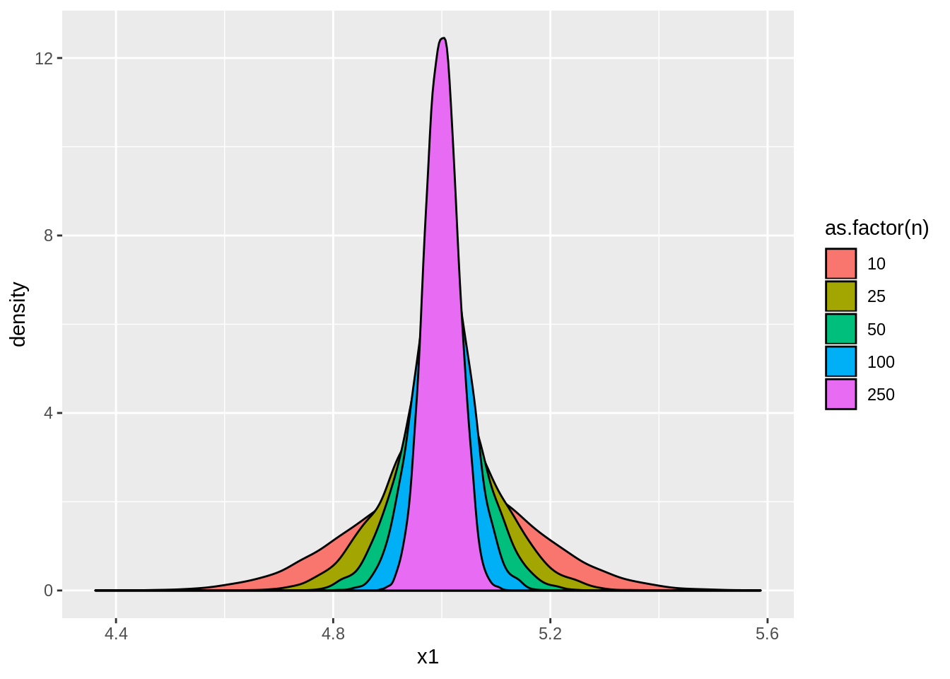
Now suppose that we want to see how having a different mean affects the sample mean. Thus we create new data, DGP2, where \[x_{1,i}\sim iid\mathcal{N}(-10,1),\;\;x_{2,i}\sim iid\mathcal{N}(0,1),\;\;\text{and}\;\;x_{3,i}\sim iid\mathcal{N}(10,1):\]
dt$x1 <- rnorm(bigN,-10,1)
dt$x2 <- rnorm(bigN,0,1)
dt$x3 <- rnorm(bigN,10,1)
Then we run the same simulation code (grouping by simulation and calculating the sample mean):
result <- dt[,lapply(.SD,mean),by=sim]We can see that the mean of the sample means is now related to the initial distribution:
result[,lapply(.SD,mean),by=n]| n | x1 | x2 | x3 |
|---|---|---|---|
| 10 | -9.999086 | -0.0077148 | 9.995435 |
| 25 | -9.998458 | -0.0001915 | 10.002076 |
| 50 | -9.998305 | -0.0006798 | 9.998413 |
| 100 | -9.998973 | -0.0019066 | 10.000033 |
| 250 | -9.998774 | 0.0005280 | 10.000636 |
But the variance of the sample means is very similar between the different data sets because \(\sigma^2=1\) in every case:
result[,lapply(.SD,var),by=n]| n | x1 | x2 | x3 |
|---|---|---|---|
| 10 | 0.0993144 | 0.1005291 | 0.1014298 |
| 25 | 0.0397848 | 0.0400464 | 0.0392695 |
| 50 | 0.0200077 | 0.0197426 | 0.0203846 |
| 100 | 0.0100375 | 0.0099725 | 0.0101591 |
| 250 | 0.0039495 | 0.0039450 | 0.0040623 |
2.4.3 Central limit theorem
Before we can discuss the central limit theorem, we need to talk about another kind of convergence, convergence in distribution. This is a weaker sort of convergence than convergence in probability. Convergence in probability says that a statistic is going to converge to a single point. Convergence in distribution says that a statistic will converge to an entire distribution and so will have some inherent randomness where a statistic which converges in probability will not. For a statistic to converge in probability, that means that in the limit there is no randomness at all. This is what the law of large numbers states. The central limit theorem gives a result which convergences in distribution which will always have some random variation from sample to sample. We define convergence in distribution as follows:
The central limit theorem is absolutely incredible. Sometimes we will want to model the distribution of the data, but whenever we don’t, we will use the central limit theorem. The theorem effectively states that we don’t have to care about the distribution of the data (beyond the existence of a mean and variance) for the sake of our statistical analysis. It is the most important theorem in statistics, and it is critical that you understand its result (not necessarily its proof which is rather time consuming and fairly obtuse).
For showing the central limit theorem, it is easiest to use smaller values of \(n\). Here we are going to let \(n=1,2,3,\) and \(5\). To show our results best we are also going to use \(100,000\) simulations instead of \(10,000\):
dt <- build.nsim(10*nsim,c(1,2,3,5))
bigN <- nrow(dt)
The data we are going to generate is from the uniform distribution \(x_i\sim iid\text{U}[-1,1]\):
dt$x <- runif(bigN,-1,1)The mean of this uniform distribution is \(0\). The variance of the uniform distribution is \(\text{Var}[x_i]=(b-a)^2/12=(1-(-1))^2/12=1/3\) so to \(z\)-transform the sample mean, we need to divide it by \(1/(3n)^{1/2}\) or equivalently, multiply it by \(\sqrt{3n}\):
zstats <- dt[,lapply(.SD,mean),by=sim]
zstats <- zstats[,.(n,x*sqrt(3*n))]
names(zstats) <- c('n','x')
Now observe the distribution of \(z\) when \(n=1\). See that \(z\) follows a uniform distribution just like our data:
ggplot(zstats[n==1],aes(x=x)) + geom_histogram(position="identity",binwidth = 0.01)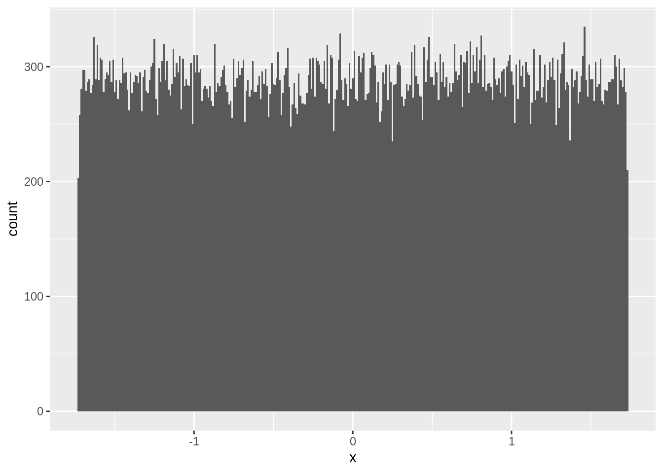
When \(n=2\), \(z\) follows a triangular distribution:
ggplot(zstats[n==2],aes(x=x)) + geom_histogram(position="identity",binwidth = 0.01)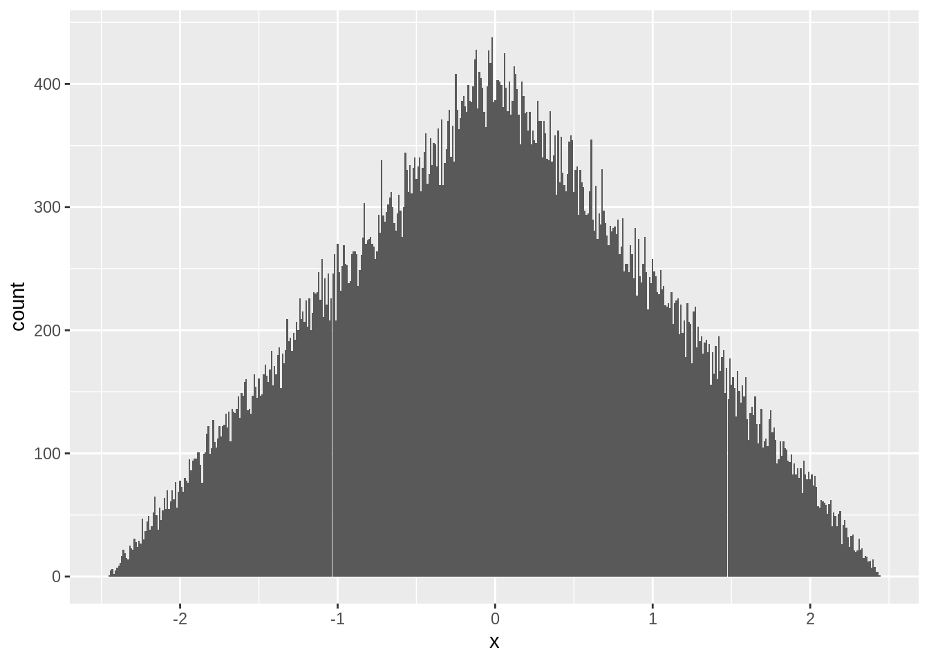
Once \(n=3\), \(z\) begins to look like a bell curve:
ggplot(zstats[n==3],aes(x=x)) + geom_histogram(position="identity",binwidth = 0.01)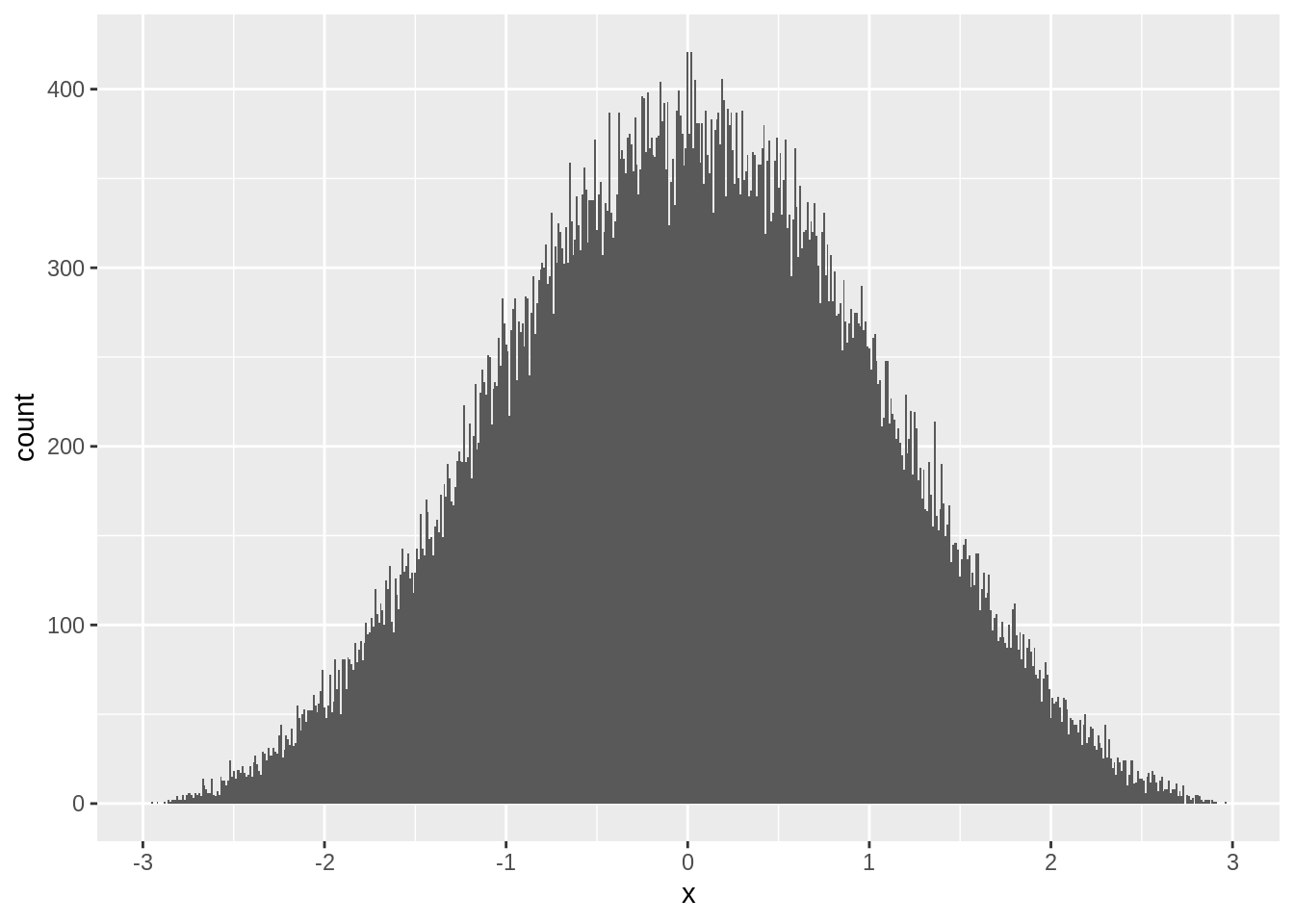
And by the time \(n=5\), \(z\) looks almost completely normal:
ggplot(zstats[n==5],aes(x=x)) + geom_histogram(position="identity",binwidth = 0.01)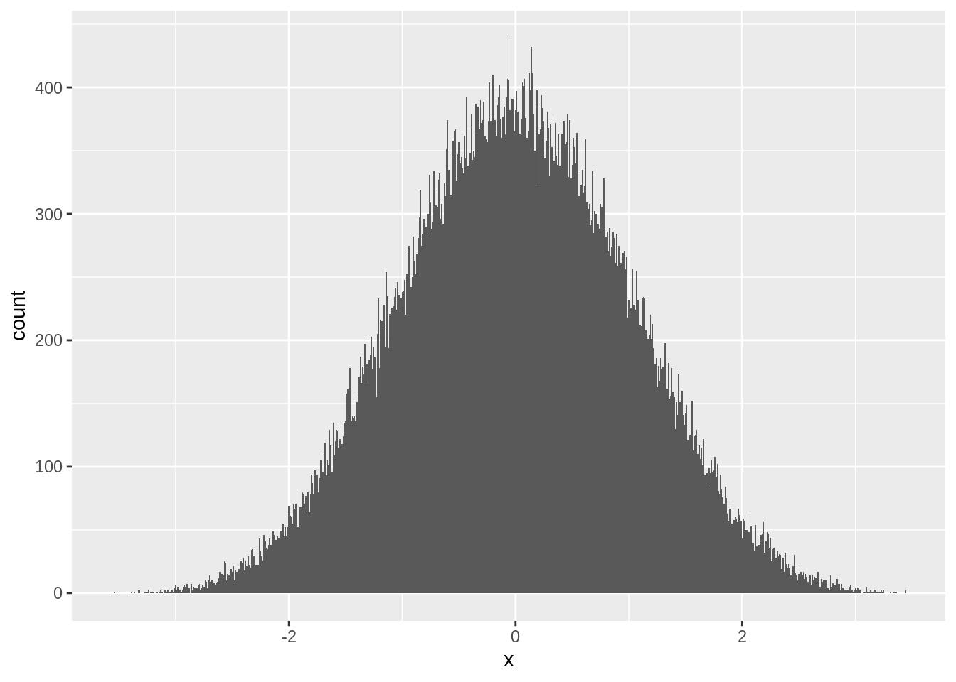
This is the result of the central limit theorem. When data is independently drawn and the sample size is large, the sample mean will always appear normally distributed:
2.4.3.1 Hypothesis testing
One direct consequence of the central limit theorem is the ability to perform hypothesis testing. First let’s start with some background information. Say we are interested in testing the hypothesis: \[\begin{aligned} \mathcal{H}_0&:\mu=5 \\ \mathcal{H}_1&:\mu\neq5 \end{aligned}\] Here the null hypothesis is that \(\mu\) is \(5\) and the alternative is that \(\mu\) is not \(5\). When we phrase a hypothesis this way, you should understand that we are trying to show the alternative hypothesis. We can never show that the null hypothesis is true, only that it is false. We are trying to show that the alternative is true. Be careful about this.
So in our case, we are interested in showing that \(\mu\neq 5\). So how do we go about this? First we construct a \(t\)-statistic: \[t=\frac{\overline{x}-5}{s/\sqrt{n}}\]
This statistic has been carefully calculated to be standardized if and only if \(\mu=5\). Let’s see how this works: \[t=\frac{\overline{x}-\mu-(5-\mu)}{s/\sqrt{n}}=\frac{\overline{x}-\mu}{s/\sqrt{n}}-\frac{5-\mu}{s/\sqrt{n}}=z\frac{\sigma}{s}-\frac{5-\mu}{s/\sqrt{n}}\]
Therefore as \(n\rightarrow\infty\), the \(\frac{5-\mu}{s/\sqrt{n}}\) term either converges to positive or negative infinity. So the \(t\)-statistic is designed to explode to either infinity or negative infinity unless \(\mu\) is actually exactly equal to \(5\). If \(\mu=5\), \(t=z\frac{\sigma}{s}\rightarrow \mathcal{N}(0,1)\) as \(n\rightarrow\infty\).
So this is our testing procedure. We calculate \(t\) which is going to be some scalar number. Then we ask, did \(t\) plausibly come from the \(\mathcal{N}(0,1)\) distribution or did it come from something that’s exploding to infinity? If \(t\) is close to \(0\), then we cannot reject the null hypothesis, so our evidence says absolutely nothing. If \(t\) is far away from \(0\), then we reject the null hypothesis, and we have good evidence.
Where do we draw the line between rejecting and accepting the null hypothesis? Because when the null is true (under the null), we know the distribution of \(t\) is asymptotically \(\mathcal{N}(0,1)\), we use this as our guide. We set some “significance level” such that a true null hypothesis will reject our test that often. So if we are using the \(5\%\) level, then we set the boundary as \(\pm 1.96\) so that when the null is true, we reject the null hypothesis in \(5\%\) of cases (this is from the normal CDF or rather its inverse).
While in a standard statistics course, you would probably be taught that we should choose some significance level and stick to it, in practice, people typically state the lowest (most significant) level that their evidence implies. The \(p\)-value tells us at what significance level we would stop rejecting the null. If the evidence points to \(5\%\) significance, then \(p<0.05\) and we will say that it is significant at the \(5\%\) level. If the evidence points to \(0.1\%\) significance, then \(p<0.001\) and we will say that it is significant at the \(0.1\%\) level. We usually stick to the basic levels: \(10\%\) \(5\%\),\(1\%\), and \(0.1\%\).
2.4.3.2 Confidence intervals
The other main consequence of the central limit theorem is the ability to construct confidence intervals. Confidence intervals can be made by reversing the process we used for hypothesis testing:
\[t=\frac{\overline{x}-\mu}{s/\sqrt{n}}\]
We are going to solve for \(\mu\) so we put \(s/\sqrt{n}\) on the left-hand side: \[t\frac{s}{\sqrt{n}}=\overline{x}-\mu\] And we isolate \(\mu\): \[\mu=\overline{x}-t \frac{s}{\sqrt{n}}\] This would work, but what are we supposed to use for \(t\) here? We are going to use the \(5\%\) critical value from the normal distribution. This gives us a \(95\%\) confidence interval: \[\overline{x}-\frac{1.96s}{\sqrt{n}}\leq\mu\leq\overline{x}+\frac{1.96s}{\sqrt{n}}\]
What this means is that as \(n\rightarrow\infty\), \(\mu\) is going to be in this interval with \(95\%\) probability, or: \[\lim_{n\rightarrow\infty}\text{Pr}\begin{bmatrix}\overline{x}-\frac{1.96s}{\sqrt{n}}\leq\mu\leq\overline{x}+\frac{1.96s}{\sqrt{n}}\end{bmatrix}=0.95\]
So we can now get confidence intervals for our estimates.
2.4.3.3 Size simulations
dt <- build.nsim(nsim,c(10,25,50,100,250))
bigN <- nrow(dt)
dt$x1 <- runif(bigN,-1,1)
dt$x2 <- runif(bigN,-0.5,0.5)
dt$x3 <- runif(bigN,-2,2)
Now we are going to calculate the \(t\)-statistics for testing the hypothesis: \[\mathcal{H}_0:\mu=0\;\;\text{against}\;\;\mathcal{H}_1:\mu\neq 0.\]
\(t\) is defined as \(\sqrt{n}\overline{x}/s_x\). In order to calculate this inside a group by, we need to execute the process in two steps. First, we divide by the standard deviation and multiply by the square-root of \(n\) while the data is still available to us. Then we group by the simulation and calculate the sample mean. Technically it might make sense to do this in the opposite order (calculating the mean first). However, once we have compressed the data down to the means, the standard deviation is harder to pull out of R. This will give us the same result:
tstats <- dt[,.(n,x1/sd(x1)*sqrt(n),x2/sd(x2)*sqrt(n),x3/sd(x3)*sqrt(n)),by=sim]
tstats <- tstats[,lapply(.SD,mean),by=sim]
names(tstats) <- c('sim','n','x1','x2','x3')
We renamed the columns in tstats to match the data. For instance, we can look at the \(t\)-statistics for x1:
ggplot(tstats,aes(x=x1,fill=as.factor(n))) + geom_density()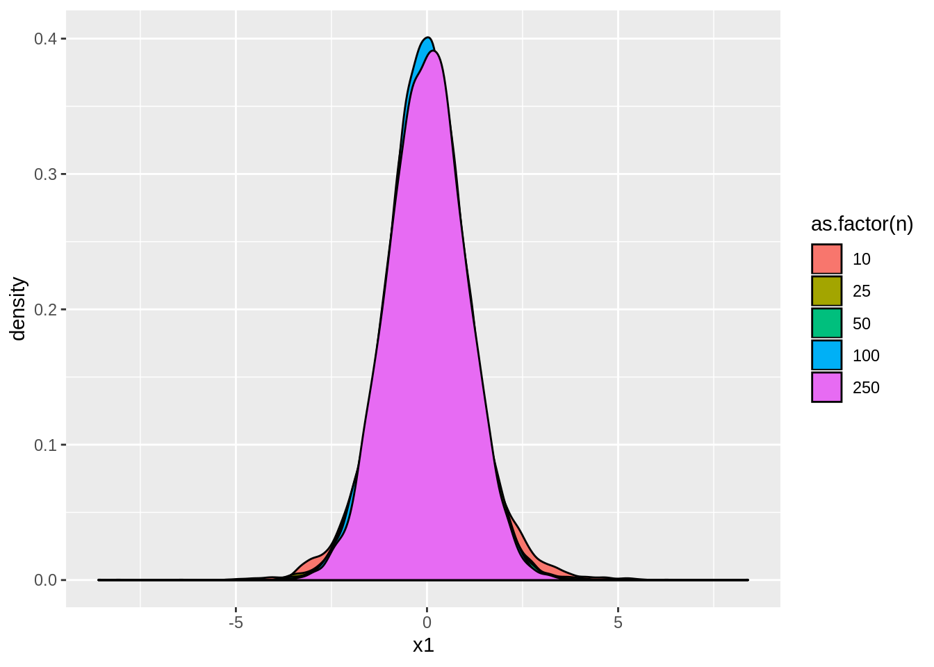
Notice that these \(t\)-statistics are normally distributed with mean \(0\) and variance around \(1\) because the null hypothesis is true. Now let’s look at the rejection rate of the hypothesis:
tstats[,.(mean(abs(x1)>1.96),mean(abs(x2)>1.96),mean(abs(x3)>1.96)),by=n]| n | x1 | x2 | x3 |
|---|---|---|---|
| 10 | 0.0862 | 0.0808 | 0.0838 |
| 25 | 0.0638 | 0.0627 | 0.0700 |
| 50 | 0.0543 | 0.0589 | 0.0540 |
| 100 | 0.0544 | 0.0519 | 0.0488 |
| 250 | 0.0493 | 0.0580 | 0.0456 |
Because the null hypothesis is true, we call this rejection rate the size of the test. The size should be around \(5\%\) because we are using \(1.96\) the critical value for the \(5\%\) test. Rejecting the null here is a mistake. Inherent in our statistical tests is a \(5\%\) error. We accept this error every time we test a hypothesis at the \(5\%\) level.
2.4.3.4 Power simulations
Now we are going to generate new data which is not centered around zero:
dt <- build.nsim(nsim,c(10,25,50,100,250))
bigN <- nrow(dt)
dt$x1 <- runif(bigN,-0.75,1)
dt$x2 <- runif(bigN,-0.5,1)
dt$x3 <- runif(bigN,-0.25,1)
In this data, the null hypothesis is going to be false. We still calculate the \(t\)-statistics exactly the same way for testing exactly the same test as above: \[\mathcal{H}_0:\mu=0\;\;\text{against}\;\;\mathcal{H}_1:\mu\neq 0.\]
tstats <- dt[,.(n,x1/sd(x1)*sqrt(n),x2/sd(x2)*sqrt(n),x3/sd(x3)*sqrt(n)),by=sim]
tstats <- tstats[,lapply(.SD,mean),by=sim]
names(tstats) <- c('sim','n','x1','x2','x3')
Now observe the distribution of \(t\). Notice that because the null is false, the distribution is no longer a \(\mathcal{N}(0,1)\):
ggplot(tstats,aes(x=x1,fill=as.factor(n))) + geom_density()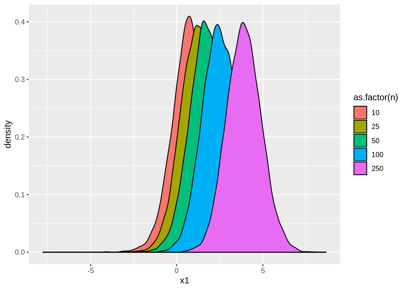
Instead, while the distribution is still approximately normal, it now moves away from \(0\) as \(n\) becomes large. If we look at the rejection rates, we find:
tstats[,.(mean(abs(x1)>1.96),mean(abs(x2)>1.96),mean(abs(x3)>1.96)),by=n]| n | x1 | x2 | x3 |
|---|---|---|---|
| 10 | 0.1442 | 0.4379 | 0.9060 |
| 25 | 0.2401 | 0.8154 | 0.9999 |
| 50 | 0.4147 | 0.9859 | 1.0000 |
| 100 | 0.6958 | 1.0000 | 1.0000 |
| 250 | 0.9756 | 1.0000 | 1.0000 |
That is, the rejection rate now approaches \(1\) as \(n\rightarrow\infty\), or in other words, we always reject the null when the sample size is large. This rejection rate is called the power of the test because the null here is false. Rejecting the null is making the correct decision about the data.
2.4.4 Sample selection bias
2.4.4.1 Bias definition
\[\text{Bias}[\hat\theta]=\text{E}[\hat\theta]-\theta\] \[\text{Bias}[\overline{x}]=\text{E}[\overline{x}]-\mu=0\]
2.4.4.2 Truncated data
2.4.4.3 Censored data
2.4.4.5 Simulation
dt <- build.nsim(nsim,c(10,25,50,100,250))
n <- nrow(dt)

dt$x <- rnorm(n,mean=0,sd=1)
dt$z <- rnorm(n,mean=0,sd=1) + dt$x/2
dt$y <- as.numeric(dt$x>0)*dt$x

result1 <- dt[,lapply(.SD,mean),by=sim]        # Basic simulation
result2 <- dt[x>=0][,lapply(.SD,mean),by=sim]  # Truncated simulation
result3 <- dt[,lapply(.SD,mean),by=sim]        # Censored simulation
result4 <- dt[z>=0][,lapply(.SD,mean),by=sim]  # Truncated on correlated variable

result1[,mean(x),by=n]
## n V1
## 1: 10 -9.673154e-05
## 2: 25 -1.559540e-03
## 3: 50 2.675015e-03
## 4: 100 -1.280059e-03
## 5: 250 1.883164e-04result2[,mean(x),by=n] ## n V1
## 1: 10 0.7909202
## 2: 25 0.7967805
## 3: 50 0.7978085
## 4: 100 0.7977201
## 5: 250 0.7972810result3[,mean(y),by=n] ## n V1
## 1: 10 0.3975853
## 2: 25 0.3978221
## 3: 50 0.3998991
## 4: 100 0.3984873
## 5: 250 0.3989139result4[,mean(x),by=n] ## n V1
## 1: 10 0.3557915
## 2: 25 0.3541482
## 3: 50 0.3574301
## 4: 100 0.3558336
## 5: 250 0.3570163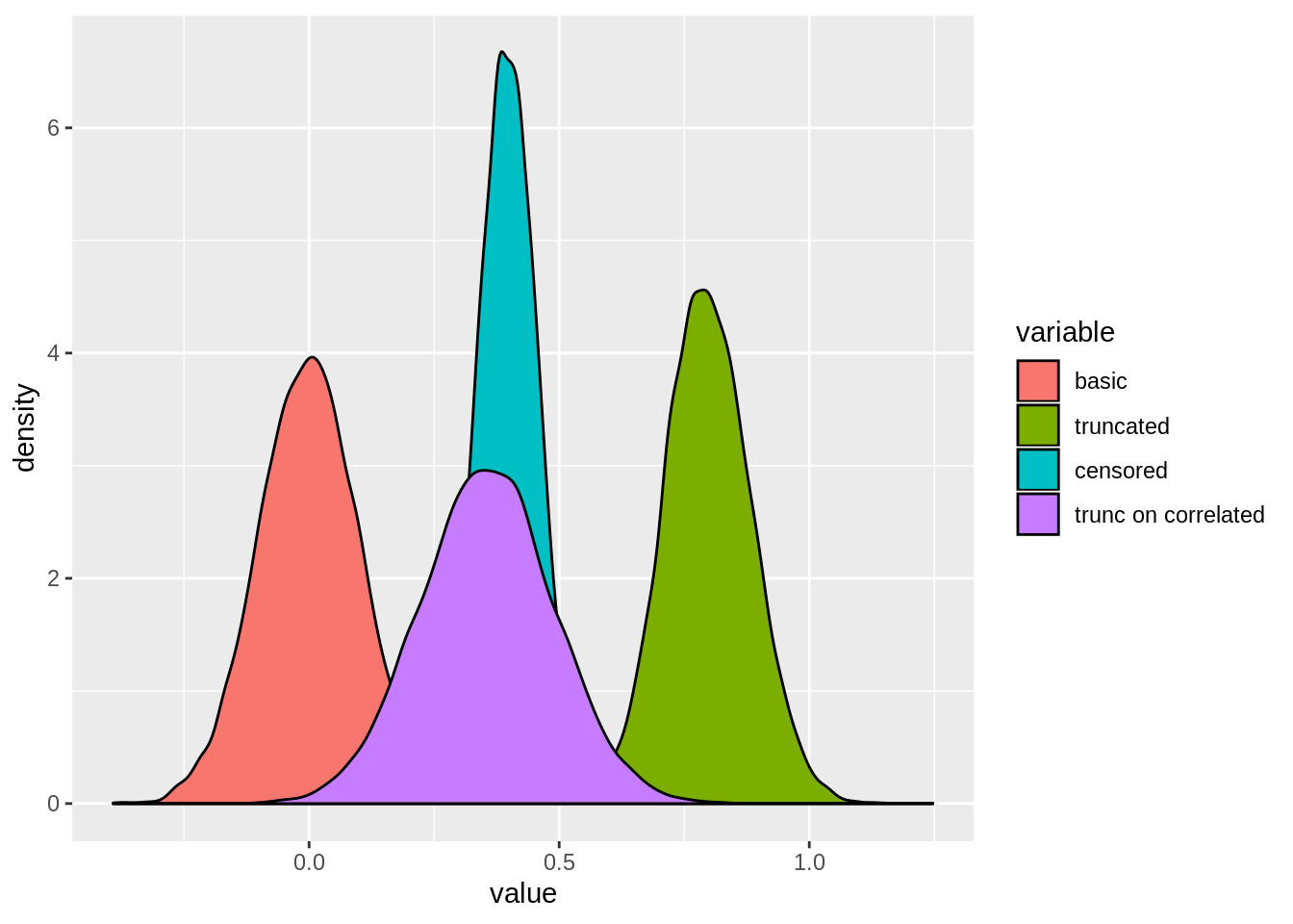
2.4.5 Maximum Likelihood
2.4.5.1 Likelihood
We have to assume some distribution to produce maximum likelihood estimates. We are going to use the normal distribution for reference, but you can choose any distribution you think the data comes from and find similar results. The normal distribution is handy because it is parameter by its population mean and variance: \[x_i \sim iid\mathcal{N}(\mu,\sigma^2)\]
Now to get the likelihood, we have to think about the joint distribution of our data: \[f(x)=f(x_1,\dots,x_n)\]
Because we made the iid independence assumption, we can find the joint distribution using the product of the marginals, or: \[f(x)=\prod_{i=1}^n f(x_i)\]
Now we can substitute the normal distribution we are familiar with: \[f(x)=\prod_{i=1}^n \frac{1}{\sqrt{2\pi\sigma^2}}\exp\begin{bmatrix}-\frac{(x_i-\mu)^2}{2\sigma^2}\end{bmatrix}\]
This joint PDF uniquely describes the data we are working with. This function is exactly identical to the likelihood function: \[L(\mu,\sigma^2|x)=\prod_{i=1}^n \frac{1}{\sqrt{2\pi\sigma^2}}\exp\begin{bmatrix}-\frac{(x_i-\mu)^2}{2\sigma^2}\end{bmatrix}\] Sometimes, this is more simply written as \(L(\mu,\sigma^2)\). What’s different about this likelihood from the joint PDF? Nothing, only the way we are thinking about it. The joint PDF tells us where the data is likely distributed given some values of \(\mu\) and \(\sigma^2\), but in practice, we don’t know \(\mu\) and \(\sigma^2\). What we do know is the data. So instead of thinking about the PDF as a function of \(x\) values, we think about it as a function of \(\mu\) and \(\sigma^2\). Then we find where \(\mu\) and \(\sigma^2\) are most likely to be by maximizing the likelihood function.
Maximum likelihood is an extremely powerful workhorse in statistics. It provides a framework for estimating unknown parameters and creating statistical tests. If you spend much time learning statistics, you will start to see maximum likelihood estimates everywhere.
Importantly you should note that \[\arg\max_{\mu,\sigma^2} L(\mu,\sigma^2) = \arg\max_{\mu,\sigma^2} \ln L(\mu,\sigma^2)\] because the natural log (or any log really) is a monotone increasing transformation. This is important because the log-likelihood is a series of sums instead of products so it is considerably easier to work with:
\[\ln L(\mu,\sigma^2)=\sum_{i=1}^n \ln\begin{bmatrix}\frac{1}{\sqrt{2\pi\sigma^2}}\end{bmatrix}-\sum_{i=1}^n \frac{(x_i-\mu)^2}{2\sigma^2}\]
Simplifying down a bit: \[\ln L(\mu,\sigma^2)=-\frac{n}{2}\ln(2\pi\sigma^2)-\frac{n}{2\sigma^2}\begin{bmatrix}n^{-1}\sum_{i=1}^n (x_i-\mu)^2\end{bmatrix}\]
2.4.5.2 Maximum likelihood
To find estimates of \(\mu\) and \(\sigma^2\), we can maximize the likelihood function with respect to these two parameters. There are many ways of maximizing a likelihood and we will study some in the optimization portion of this chapter, but the most direct way is using calculus. To find the maximum or minimum of a function in calculus, we are going to take the derivative and set the derivative equal to zero to find where the function is flat. That means producing the following first-order conditions:
\[\begin{aligned} \frac{d}{d\mu}\ln L(\mu,\sigma^2)&=0 \\ \frac{d}{d\sigma^2}\ln L(\mu,\sigma^2)&=0 \end{aligned}\]
In our case where we know the log-likelihood: \[\begin{aligned} \frac{d}{d\mu}\ln L(\mu,\sigma^2)&=\frac{n}{\sigma^2}\begin{bmatrix}n^{-1}\sum_{i=1}^n (x_i-\mu)\end{bmatrix} \\ \frac{d}{d\sigma^2}\ln L(\mu,\sigma^2)&=-\frac{n}{2\sigma^2}+\frac{n}{2\sigma^4}\begin{bmatrix}n^{-1}\sum_{i=1}^n (x_i-\mu)^2\end{bmatrix} \end{aligned}\]
Or simplifying these equations and solving for \(\mu\) and \(\sigma^2\): \[\begin{aligned} 0&=n^{-1}\sum_{i=1}^n (x_i-\hat\mu)\;\text{or}\;\hat\mu=\overline x \\ \hat\sigma^2&=n^{-1}\sum_{i=1}^n (x_i-\hat\mu)^2\;\text{or}\;\hat\sigma^2=n^{-1}\sum_{i=1}^n (x_i-\overline x)^2 \end{aligned}\]
2.4.5.3 Expected value of the ML estimates
\[\text{E}[\hat\sigma^2]=\text{E}[n^{-1}\sum_{i=1}^n (x_i-\overline x)^2]\]
\[\text{E}[\hat\sigma^2]=\text{E}[n^{-1}\sum_{i=1}^n (x_i-\mu-(\overline x-\mu))^2]\]
\[\text{E}[\hat\sigma^2]=\text{E}\begin{bmatrix}n^{-1}\sum_{i=1}^n \begin{bmatrix}(x_i-\mu)^2-2(\overline x-\mu)(x_i-\mu)+(\overline x-\mu)^2\end{bmatrix}\end{bmatrix}\]
\[\text{E}[\hat\sigma^2]=\text{E}\begin{bmatrix}n^{-1}\sum_{i=1}^n (x_i-\mu)^2\end{bmatrix}-\text{E}\begin{bmatrix}(\overline x-\mu)^2\end{bmatrix}\]
\[\text{E}[\hat\sigma^2]=\text{Var}[x_i]-\text{Var}[\overline x]\] \[\text{E}[\hat\sigma^2]=\sigma^2-\frac{\sigma^2}{n}\] \[\text{E}[\hat\sigma^2]=\sigma^2\frac{n-1}{n}\]
This means that the maximum likelihood estimator of the variance is biased because \(\text{E}[\hat\sigma^2]\neq \sigma^2\). The estimator is still consistent because as \(n\rightarrow\infty\), \(\text{E}[\hat\sigma^2]\rightarrow \sigma^2\), but it is biased in finite samples. This also mean that \(\text{E}[s^2]=\sigma^2\) which is why we defined \(s^2\) as we did. By dividing by \(n-1\), \(s^2\) is the unbiased estimator of the population variance.
2.4.5.4 Bias-variance trade-off
Consider the bias of our maximum likelihood estimate: \[\text{Bias}[\hat\sigma^2]=\text{E}[\hat\sigma^2]-\sigma^2=-\frac{\sigma^2}{n}\neq 0\] This is not equal to zero, but the bias of \(s^2\) is: \[\text{Bias}[s^2]=\text{E}[s^2]-\sigma^2=0\] So we know that \(\hat\sigma^2\) has a large absolute bias than \(s^2\). But by our properties of the variance, and the fact that we know that \(\hat\sigma^2=s^2\frac{n-1}{n}\), \[\text{Var}[\hat\sigma^2]=Var[s^2]\frac{(n-1)^2}{n^2}\] This means that \(\hat\sigma^2\) has a smaller variance than \(s^2\). This is known as the bias-variance trade-off and is a common theme in statistics. On one hand we could use the unbiased version, \(s^2\), but this has a larger variance. Or we could use the small variance estimator \(\hat\sigma^2\), but this is biased. So which one should we use? Here, it really doesn’t matter because \(s^2\approx\hat\sigma^2\) for large values of \(n\) like the data we are going to be working with. But in other cases this is a more serious problem, and we will be talking about some of those later in the book.