3.2 Model selection and endogeneity
3.2.1 Maximum likelihood
3.2.2 Model selection criteria
Consider the bwght example from Chapter ??. Suppose we run the following model:
model1 <- lm(log(bwght)~cigs+faminc+male+white+motheduc+fatheduc,data=bwght)I am using complete.cases here because the following methods are not robust to missing values (which complete.cases drops). To compute the Akaike information criterion (AIC) of the model, simply type:
AIC(model1)## [1] -638.222Similarly to get the BIC, use the BIC function.
3.2.3 Step-wise regression
To use step-wise regression to simplify the model by finding the lowest AIC value, just type:
model2 <- step(model1)Alternatively, we can find the best model using the BIC by adding
model3 <- step(model1,k=log(nrow(bwght)))Note that because we specified \(k=\ln(n)\), we know this is using the BIC even though the output says AIC.
3.2.4 A note on hypothesis testing
3.2.5 Endogeneity definition
3.2.5.1 Expected value of the coefficients
3.2.5.2 Exogeneity assumption
3.2.5.3 Unbiased simulation
We covered the build.nsim function in chapter ??:
dt <- build.nsim(nsim,c(10,25,50,100,250))
bigN <- nrow(dt)
Once the collections of simulation environment is created, we need to generate some data. For this, we can set up a few basic variables, dt$x and dt$y:
dt$x <- rnorm(bigN,2,1)
dt$y <- 2*dt$x + rnorm(bigN,0,1)
Here, \(x_i\sim iid\mathcal N(2,1)\) and \(e_i\sim iid\mathcal N(0,1)\) and \[y_i=\beta_1 x_i + e_i = 2x_i+e_i\]. Next we can run the linear models. The issue is that in order to do this inside our group-by statement, we need to output the result in some tidy format. Sometimes, we might be interest in simulating the glance statistics:
dt[,glance(lm(y~x)),by=.(n,sim)]## n sim r.squared adj.r.squared sigma statistic p.value
## 1: 10 1 0.7905678 0.7643888 1.0791416 30.19852 5.769226e-04
## 2: 10 2 0.7803381 0.7528803 1.1099545 28.41960 7.016822e-04
## 3: 10 3 0.8025502 0.7778689 1.0611060 32.51662 4.531588e-04
## 4: 10 4 0.8521860 0.8337092 0.9665015 46.12207 1.390489e-04
## 5: 10 5 0.6918718 0.6533557 1.1480775 17.96322 2.844030e-03
## ---
## 49996: 250 49996 0.7926300 0.7917938 1.0153844 947.92974 1.073480e-86
## 49997: 250 49997 0.8283488 0.8276566 0.9684280 1196.79010 6.934725e-97
## 49998: 250 49998 0.8094907 0.8087225 1.0152319 1053.77373 2.879841e-91
## 49999: 250 49999 0.7974613 0.7966446 0.9822531 976.45741 5.754041e-88
## 50000: 250 50000 0.7894579 0.7886089 1.0259765 929.91148 7.066252e-86
## df logLik AIC BIC deviance df.residual
## 1: 2 -13.83533 33.67065 34.57841 9.316372 8
## 2: 2 -14.11686 34.23371 35.14147 9.855991 8
## 3: 2 -13.66679 33.33357 34.24133 9.007568 8
## 4: 2 -12.73294 31.46589 32.37364 7.473002 8
## 5: 2 -14.45456 34.90911 35.81687 10.544655 8
## ---
## 49996: 2 -357.54742 721.09484 731.65923 255.689348 248
## 49997: 2 -345.71032 697.42063 707.98501 232.587472 248
## 49998: 2 -357.50988 721.01977 731.58415 255.612577 248
## 49999: 2 -349.25406 704.50812 715.07250 239.275669 248
## 50000: 2 -360.14181 726.28363 736.84801 261.051672 248Here, we are interested in obtaining the estimated \(\beta_1\) coefficients:
result <- dt[,tidy(lm(y~x))[2,],by=.(n,sim)]
result
## n sim term estimate std.error statistic p.value
## 1: 10 1 x 1.522488 0.27705177 5.495318 5.769226e-04
## 2: 10 2 x 1.893609 0.35520678 5.331004 7.016822e-04
## 3: 10 3 x 2.094013 0.36722029 5.702335 4.531588e-04
## 4: 10 4 x 2.415660 0.35569795 6.791323 1.390489e-04
## 5: 10 5 x 2.200994 0.51931009 4.238303 2.844030e-03
## ---
## 49996: 250 49996 x 2.049229 0.06655834 30.788468 1.073480e-86
## 49997: 250 49997 x 2.095238 0.06056537 34.594654 6.934725e-97
## 49998: 250 49998 x 2.005738 0.06178749 32.461881 2.879841e-91
## 49999: 250 49999 x 1.933262 0.06186771 31.248319 5.754041e-88
## 50000: 250 50000 x 2.070814 0.06790789 30.494450 7.066252e-86This gives us 5000 different \(\hat\beta_1\) values. We can then group-by the sample size used to find the mean and variance of \(\hat\beta_1\):
result[,.(mean(estimate),var(estimate)),by=n]## n V1 V2
## 1: 10 1.996826 0.143108233
## 2: 25 2.000226 0.045006980
## 3: 50 2.002831 0.021289006
## 4: 100 2.000351 0.010120972
## 5: 250 1.999203 0.003926791You can clean up the results by creating the following function:
tab.sim <- function(dtinput,column=quote(estimate)){
  dt <- dtinput[,.(mean(eval(column)),var(eval(column))),by=n]
  names(dt) <- c("n","mean","variance")
  return(dt)
}tab.sim(result)| n | mean | variance |
|---|---|---|
| 10 | 1.996826 | 0.1431082 |
| 25 | 2.000226 | 0.0450070 |
| 50 | 2.002831 | 0.0212890 |
| 100 | 2.000351 | 0.0101210 |
| 250 | 1.999203 | 0.0039268 |
Notice that the \(\hat\beta_1\) values from the model without endogeneity are centered around \(\beta_1=2\) with a variance that approaches zero as \(n\rightarrow\infty\).
3.2.6 Sources of endogeneity
3.2.6.1 Sample selection bias
3.2.6.2 Omitted variable bias
dt$w <- rnorm(bigN,0,0.5)
dt$x <- rnorm(bigN,2,0.5) + dt$w
dt$z <- rnorm(bigN,1,0.5) + dt$w
dt$y <- 2*dt$x + 3*dt$z + rnorm(bigN,0,1)
result <- dt[,tidy(lm(y~x))[2,],by=.(n,sim)]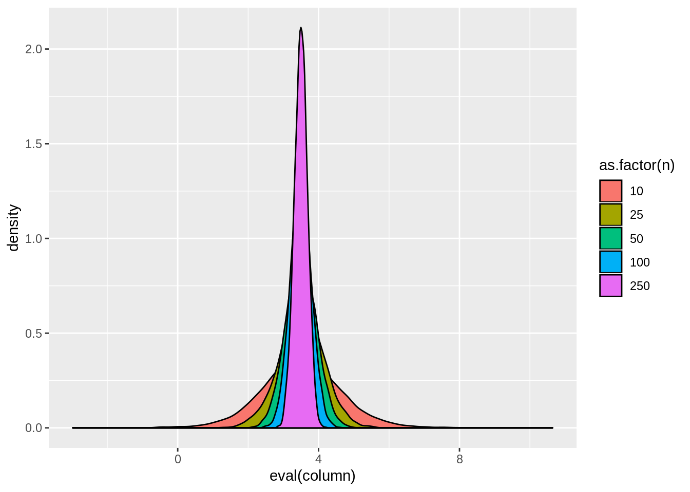
result <- dt[,tidy(lm(y~x))[2,],by=.(n,sim)]
tab.sim(result)| n | mean | variance |
|---|---|---|
| 10 | 3.510818 | 1.2778899 |
| 25 | 3.508936 | 0.3905536 |
| 50 | 3.502884 | 0.1853704 |
| 100 | 3.497456 | 0.0902560 |
| 250 | 3.498624 | 0.0357755 |
3.2.6.3 Outlier bias
3.2.6.4 Measurement error bias
dt$x <- rnorm(bigN,2,1)
dt$xstar <- dt$x + rnorm(bigN,0,1)
dt$y <- 2*dt$x + rnorm(bigN,0,1)
dt$ystar <- dt$y + rnorm(bigN,0,1)
tab.sim(dt[,tidy(lm(ystar~xstar))[2,],by=.(n,sim)])
## n mean variance
## 1: 10 0.9996409 0.287528741
## 2: 25 1.0017050 0.089506290
## 3: 50 1.0000425 0.042499906
## 4: 100 0.9974228 0.020793890
## 5: 250 1.0007813 0.008082634tab.sim(dt[,tidy(lm(y~xstar))[2,],by=.(n,sim)])## n mean variance
## 1: 10 1.0007801 0.215746414
## 2: 25 1.0017694 0.067357052
## 3: 50 1.0008632 0.031392542
## 4: 100 0.9981413 0.015638762
## 5: 250 1.0007376 0.006033224tab.sim(dt[,tidy(lm(ystar~x))[2,],by=.(n,sim)])## n mean variance
## 1: 10 2.003924 0.286280370
## 2: 25 2.003591 0.090385638
## 3: 50 1.999744 0.042309487
## 4: 100 1.996857 0.020447698
## 5: 250 2.000420 0.0081247843.2.6.5 Reverse regression bias
dt$x <- rnorm(bigN,2,1)
dt$y <- 2*dt$x + rnorm(bigN,0,1)
result <- dt[,tidy(lm(x~y))[2,],by=.(n,sim)]
result$estimate <- 1/result$estimate
tab.sim(result[estimate<5])
## n mean variance
## 1: 10 2.577353 0.255151301
## 2: 25 2.527498 0.075751517
## 3: 50 2.515748 0.035413432
## 4: 100 2.505908 0.016630351
## 5: 250 2.502658 0.006385136